%%html
<script src="https://bits.csb.pitt.edu/preamble.js"></script>
What is clustering?
Wikipedia: Cluster analysis or clustering is the task of grouping a set of objects in such a way that objects in the same group (called a cluster) are more similar (in some sense or another) to each other than to those in other groups (clusters).
Generally speaking, clustering is NP-hard, so it is difficult to identify a provable optimal clustering.

What is similar?
- similarity: larger number means more similar
- Tanimoto (or Jaccard) similarity of two sets: $$\frac{|A \cap B|}{|A \cup B|}$$
- distance: larger number means less similar (zero means identical)
- Euclidean distance (L2 norm) between $n$-dimensional vectors $u$ and $v$: $$\|u - v\|_2 = \sqrt{\sum_i^n (u_i - v_i)^2}$$
- Cityblock (Manhattan) distance (L1 norm): $$\|u - v\|_1 = \sum_i^n|u_i - v_i|$$
- Cosine distance between $n$-dimensional vectors $u$ and $v$: $$1 - \frac{u \cdot v}{\|u\|_2 \|v\|_2}$$
%%html
<div id="tanimotosim" style="width: 500px"></div>
<script>
$('head').append('<link rel="stylesheet" href="https://bits.csb.pitt.edu/asker.js/themes/asker.default.css" />');

    var divid = '#tanimotosim';
	jQuery(divid).asker({
	    id: divid,
	    question: "What is the range for Tanimoto similarity?",
		answers: ['0...1','-inf...inf','0...inf','-1...1'],
        server: "https://bits.csb.pitt.edu/asker.js/example/asker.cgi",
		charter: chartmaker})

$(".jp-InputArea .o:contains(html)").closest('.jp-InputArea').hide();


</script>
Given two vectors $u = (0,1)$ and $v = (2,0)$
%%html
<div id="euclideanuv" style="width: 500px"></div>
<script>
$('head').append('<link rel="stylesheet" href="https://bits.csb.pitt.edu/asker.js/themes/asker.default.css" />');

    var divid = '#euclideanuv';
	jQuery(divid).asker({
	    id: divid,
	    question: "What Euclidean distance between u and v?",
		answers: ['0','1','2','2.23','3','5'],
        server: "https://bits.csb.pitt.edu/asker.js/example/asker.cgi",
		charter: chartmaker})

$(".jp-InputArea .o:contains(html)").closest('.jp-InputArea').hide();


</script>
Given two vectors $u = (0,1)$ and $v = (2,0)$
%%html
<div id="cityblockuv" style="width: 500px"></div>
<script>
$('head').append('<link rel="stylesheet" href="https://bits.csb.pitt.edu/asker.js/themes/asker.default.css" />');

    var divid = '#cityblockuv';
	jQuery(divid).asker({
	    id: divid,
	    question: "What cityblock distance between u and v?",
		answers: ['0','1','2','2.23','3','5'],
        server: "https://bits.csb.pitt.edu/asker.js/example/asker.cgi",
		charter: chartmaker})

$(".jp-InputArea .o:contains(html)").closest('.jp-InputArea').hide();


</script>
Given two vectors $u = (0,1)$ and $v = (2,0)$
%%html
<div id="cosineuv" style="width: 500px"></div>
<script>
$('head').append('<link rel="stylesheet" href="https://bits.csb.pitt.edu/asker.js/themes/asker.default.css" />');

    var divid = '#cosineuv';
	jQuery(divid).asker({
	    id: divid,
	    question: "What cosine distance between u and v?",
		answers: ['0','1','2','2.23','3','5'],
        server: "https://bits.csb.pitt.edu/asker.js/example/asker.cgi",
		charter: chartmaker})

$(".jp-InputArea .o:contains(html)").closest('.jp-InputArea').hide();


</script>
import scipy.spatial.distance
help(scipy.spatial.distance)
Help on module scipy.spatial.distance in scipy.spatial:
NAME
scipy.spatial.distance
DESCRIPTION
Distance computations (:mod:`scipy.spatial.distance`)
=====================================================
.. sectionauthor:: Damian Eads
Function reference
------------------
Distance matrix computation from a collection of raw observation vectors
stored in a rectangular array.
.. autosummary::
:toctree: generated/
pdist -- pairwise distances between observation vectors.
cdist -- distances between two collections of observation vectors
squareform -- convert distance matrix to a condensed one and vice versa
directed_hausdorff -- directed Hausdorff distance between arrays
Predicates for checking the validity of distance matrices, both
condensed and redundant. Also contained in this module are functions
for computing the number of observations in a distance matrix.
.. autosummary::
:toctree: generated/
is_valid_dm -- checks for a valid distance matrix
is_valid_y -- checks for a valid condensed distance matrix
num_obs_dm -- # of observations in a distance matrix
num_obs_y -- # of observations in a condensed distance matrix
Distance functions between two numeric vectors ``u`` and ``v``. Computing
distances over a large collection of vectors is inefficient for these
functions. Use ``pdist`` for this purpose.
.. autosummary::
:toctree: generated/
braycurtis -- the Bray-Curtis distance.
canberra -- the Canberra distance.
chebyshev -- the Chebyshev distance.
cityblock -- the Manhattan distance.
correlation -- the Correlation distance.
cosine -- the Cosine distance.
euclidean -- the Euclidean distance.
jensenshannon -- the Jensen-Shannon distance.
mahalanobis -- the Mahalanobis distance.
minkowski -- the Minkowski distance.
seuclidean -- the normalized Euclidean distance.
sqeuclidean -- the squared Euclidean distance.
Distance functions between two boolean vectors (representing sets) ``u`` and
``v``. As in the case of numerical vectors, ``pdist`` is more efficient for
computing the distances between all pairs.
.. autosummary::
:toctree: generated/
dice -- the Dice dissimilarity.
hamming -- the Hamming distance.
jaccard -- the Jaccard distance.
kulczynski1 -- the Kulczynski 1 distance.
rogerstanimoto -- the Rogers-Tanimoto dissimilarity.
russellrao -- the Russell-Rao dissimilarity.
sokalmichener -- the Sokal-Michener dissimilarity.
sokalsneath -- the Sokal-Sneath dissimilarity.
yule -- the Yule dissimilarity.
:func:`hamming` also operates over discrete numerical vectors.
FUNCTIONS
braycurtis(u, v, w=None)
Compute the Bray-Curtis distance between two 1-D arrays.
Bray-Curtis distance is defined as
.. math::
\sum{|u_i-v_i|} / \sum{|u_i+v_i|}
The Bray-Curtis distance is in the range [0, 1] if all coordinates are
positive, and is undefined if the inputs are of length zero.
Parameters
----------
u : (N,) array_like
Input array.
v : (N,) array_like
Input array.
w : (N,) array_like, optional
The weights for each value in `u` and `v`. Default is None,
which gives each value a weight of 1.0
Returns
-------
braycurtis : double
The Bray-Curtis distance between 1-D arrays `u` and `v`.
Examples
--------
>>> from scipy.spatial import distance
>>> distance.braycurtis([1, 0, 0], [0, 1, 0])
1.0
>>> distance.braycurtis([1, 1, 0], [0, 1, 0])
0.33333333333333331
canberra(u, v, w=None)
Compute the Canberra distance between two 1-D arrays.
The Canberra distance is defined as
.. math::
d(u,v) = \sum_i \frac{|u_i-v_i|}
{|u_i|+|v_i|}.
Parameters
----------
u : (N,) array_like
Input array.
v : (N,) array_like
Input array.
w : (N,) array_like, optional
The weights for each value in `u` and `v`. Default is None,
which gives each value a weight of 1.0
Returns
-------
canberra : double
The Canberra distance between vectors `u` and `v`.
Notes
-----
When `u[i]` and `v[i]` are 0 for given i, then the fraction 0/0 = 0 is
used in the calculation.
Examples
--------
>>> from scipy.spatial import distance
>>> distance.canberra([1, 0, 0], [0, 1, 0])
2.0
>>> distance.canberra([1, 1, 0], [0, 1, 0])
1.0
cdist(XA, XB, metric='euclidean', *, out=None, **kwargs)
Compute distance between each pair of the two collections of inputs.
See Notes for common calling conventions.
Parameters
----------
XA : array_like
An :math:`m_A` by :math:`n` array of :math:`m_A`
original observations in an :math:`n`-dimensional space.
Inputs are converted to float type.
XB : array_like
An :math:`m_B` by :math:`n` array of :math:`m_B`
original observations in an :math:`n`-dimensional space.
Inputs are converted to float type.
metric : str or callable, optional
The distance metric to use. If a string, the distance function can be
'braycurtis', 'canberra', 'chebyshev', 'cityblock', 'correlation',
'cosine', 'dice', 'euclidean', 'hamming', 'jaccard', 'jensenshannon',
'kulczynski1', 'mahalanobis', 'matching', 'minkowski',
'rogerstanimoto', 'russellrao', 'seuclidean', 'sokalmichener',
'sokalsneath', 'sqeuclidean', 'yule'.
**kwargs : dict, optional
Extra arguments to `metric`: refer to each metric documentation for a
list of all possible arguments.
Some possible arguments:
p : scalar
The p-norm to apply for Minkowski, weighted and unweighted.
Default: 2.
w : array_like
The weight vector for metrics that support weights (e.g., Minkowski).
V : array_like
The variance vector for standardized Euclidean.
Default: var(vstack([XA, XB]), axis=0, ddof=1)
VI : array_like
The inverse of the covariance matrix for Mahalanobis.
Default: inv(cov(vstack([XA, XB].T))).T
out : ndarray
The output array
If not None, the distance matrix Y is stored in this array.
Returns
-------
Y : ndarray
A :math:`m_A` by :math:`m_B` distance matrix is returned.
For each :math:`i` and :math:`j`, the metric
``dist(u=XA[i], v=XB[j])`` is computed and stored in the
:math:`ij` th entry.
Raises
------
ValueError
An exception is thrown if `XA` and `XB` do not have
the same number of columns.
Notes
-----
The following are common calling conventions:
1. ``Y = cdist(XA, XB, 'euclidean')``
Computes the distance between :math:`m` points using
Euclidean distance (2-norm) as the distance metric between the
points. The points are arranged as :math:`m`
:math:`n`-dimensional row vectors in the matrix X.
2. ``Y = cdist(XA, XB, 'minkowski', p=2.)``
Computes the distances using the Minkowski distance
:math:`\|u-v\|_p` (:math:`p`-norm) where :math:`p > 0` (note
that this is only a quasi-metric if :math:`0 < p < 1`).
3. ``Y = cdist(XA, XB, 'cityblock')``
Computes the city block or Manhattan distance between the
points.
4. ``Y = cdist(XA, XB, 'seuclidean', V=None)``
Computes the standardized Euclidean distance. The standardized
Euclidean distance between two n-vectors ``u`` and ``v`` is
.. math::
\sqrt{\sum {(u_i-v_i)^2 / V[x_i]}}.
V is the variance vector; V[i] is the variance computed over all
the i'th components of the points. If not passed, it is
automatically computed.
5. ``Y = cdist(XA, XB, 'sqeuclidean')``
Computes the squared Euclidean distance :math:`\|u-v\|_2^2` between
the vectors.
6. ``Y = cdist(XA, XB, 'cosine')``
Computes the cosine distance between vectors u and v,
.. math::
1 - \frac{u \cdot v}
{{\|u\|}_2 {\|v\|}_2}
where :math:`\|*\|_2` is the 2-norm of its argument ``*``, and
:math:`u \cdot v` is the dot product of :math:`u` and :math:`v`.
7. ``Y = cdist(XA, XB, 'correlation')``
Computes the correlation distance between vectors u and v. This is
.. math::
1 - \frac{(u - \bar{u}) \cdot (v - \bar{v})}
{{\|(u - \bar{u})\|}_2 {\|(v - \bar{v})\|}_2}
where :math:`\bar{v}` is the mean of the elements of vector v,
and :math:`x \cdot y` is the dot product of :math:`x` and :math:`y`.
8. ``Y = cdist(XA, XB, 'hamming')``
Computes the normalized Hamming distance, or the proportion of
those vector elements between two n-vectors ``u`` and ``v``
which disagree. To save memory, the matrix ``X`` can be of type
boolean.
9. ``Y = cdist(XA, XB, 'jaccard')``
Computes the Jaccard distance between the points. Given two
vectors, ``u`` and ``v``, the Jaccard distance is the
proportion of those elements ``u[i]`` and ``v[i]`` that
disagree where at least one of them is non-zero.
10. ``Y = cdist(XA, XB, 'jensenshannon')``
Computes the Jensen-Shannon distance between two probability arrays.
Given two probability vectors, :math:`p` and :math:`q`, the
Jensen-Shannon distance is
.. math::
\sqrt{\frac{D(p \parallel m) + D(q \parallel m)}{2}}
where :math:`m` is the pointwise mean of :math:`p` and :math:`q`
and :math:`D` is the Kullback-Leibler divergence.
11. ``Y = cdist(XA, XB, 'chebyshev')``
Computes the Chebyshev distance between the points. The
Chebyshev distance between two n-vectors ``u`` and ``v`` is the
maximum norm-1 distance between their respective elements. More
precisely, the distance is given by
.. math::
d(u,v) = \max_i {|u_i-v_i|}.
12. ``Y = cdist(XA, XB, 'canberra')``
Computes the Canberra distance between the points. The
Canberra distance between two points ``u`` and ``v`` is
.. math::
d(u,v) = \sum_i \frac{|u_i-v_i|}
{|u_i|+|v_i|}.
13. ``Y = cdist(XA, XB, 'braycurtis')``
Computes the Bray-Curtis distance between the points. The
Bray-Curtis distance between two points ``u`` and ``v`` is
.. math::
d(u,v) = \frac{\sum_i (|u_i-v_i|)}
{\sum_i (|u_i+v_i|)}
14. ``Y = cdist(XA, XB, 'mahalanobis', VI=None)``
Computes the Mahalanobis distance between the points. The
Mahalanobis distance between two points ``u`` and ``v`` is
:math:`\sqrt{(u-v)(1/V)(u-v)^T}` where :math:`(1/V)` (the ``VI``
variable) is the inverse covariance. If ``VI`` is not None,
``VI`` will be used as the inverse covariance matrix.
15. ``Y = cdist(XA, XB, 'yule')``
Computes the Yule distance between the boolean
vectors. (see `yule` function documentation)
16. ``Y = cdist(XA, XB, 'matching')``
Synonym for 'hamming'.
17. ``Y = cdist(XA, XB, 'dice')``
Computes the Dice distance between the boolean vectors. (see
`dice` function documentation)
18. ``Y = cdist(XA, XB, 'kulczynski1')``
Computes the kulczynski distance between the boolean
vectors. (see `kulczynski1` function documentation)
19. ``Y = cdist(XA, XB, 'rogerstanimoto')``
Computes the Rogers-Tanimoto distance between the boolean
vectors. (see `rogerstanimoto` function documentation)
20. ``Y = cdist(XA, XB, 'russellrao')``
Computes the Russell-Rao distance between the boolean
vectors. (see `russellrao` function documentation)
21. ``Y = cdist(XA, XB, 'sokalmichener')``
Computes the Sokal-Michener distance between the boolean
vectors. (see `sokalmichener` function documentation)
22. ``Y = cdist(XA, XB, 'sokalsneath')``
Computes the Sokal-Sneath distance between the vectors. (see
`sokalsneath` function documentation)
23. ``Y = cdist(XA, XB, f)``
Computes the distance between all pairs of vectors in X
using the user supplied 2-arity function f. For example,
Euclidean distance between the vectors could be computed
as follows::
dm = cdist(XA, XB, lambda u, v: np.sqrt(((u-v)**2).sum()))
Note that you should avoid passing a reference to one of
the distance functions defined in this library. For example,::
dm = cdist(XA, XB, sokalsneath)
would calculate the pair-wise distances between the vectors in
X using the Python function `sokalsneath`. This would result in
sokalsneath being called :math:`{n \choose 2}` times, which
is inefficient. Instead, the optimized C version is more
efficient, and we call it using the following syntax::
dm = cdist(XA, XB, 'sokalsneath')
Examples
--------
Find the Euclidean distances between four 2-D coordinates:
>>> from scipy.spatial import distance
>>> import numpy as np
>>> coords = [(35.0456, -85.2672),
... (35.1174, -89.9711),
... (35.9728, -83.9422),
... (36.1667, -86.7833)]
>>> distance.cdist(coords, coords, 'euclidean')
array([[ 0. , 4.7044, 1.6172, 1.8856],
[ 4.7044, 0. , 6.0893, 3.3561],
[ 1.6172, 6.0893, 0. , 2.8477],
[ 1.8856, 3.3561, 2.8477, 0. ]])
Find the Manhattan distance from a 3-D point to the corners of the unit
cube:
>>> a = np.array([[0, 0, 0],
... [0, 0, 1],
... [0, 1, 0],
... [0, 1, 1],
... [1, 0, 0],
... [1, 0, 1],
... [1, 1, 0],
... [1, 1, 1]])
>>> b = np.array([[ 0.1, 0.2, 0.4]])
>>> distance.cdist(a, b, 'cityblock')
array([[ 0.7],
[ 0.9],
[ 1.3],
[ 1.5],
[ 1.5],
[ 1.7],
[ 2.1],
[ 2.3]])
chebyshev(u, v, w=None)
Compute the Chebyshev distance.
Computes the Chebyshev distance between two 1-D arrays `u` and `v`,
which is defined as
.. math::
\max_i {|u_i-v_i|}.
Parameters
----------
u : (N,) array_like
Input vector.
v : (N,) array_like
Input vector.
w : (N,) array_like, optional
Unused, as 'max' is a weightless operation. Here for API consistency.
Returns
-------
chebyshev : double
The Chebyshev distance between vectors `u` and `v`.
Examples
--------
>>> from scipy.spatial import distance
>>> distance.chebyshev([1, 0, 0], [0, 1, 0])
1
>>> distance.chebyshev([1, 1, 0], [0, 1, 0])
1
cityblock(u, v, w=None)
Compute the City Block (Manhattan) distance.
Computes the Manhattan distance between two 1-D arrays `u` and `v`,
which is defined as
.. math::
\sum_i {\left| u_i - v_i \right|}.
Parameters
----------
u : (N,) array_like
Input array.
v : (N,) array_like
Input array.
w : (N,) array_like, optional
The weights for each value in `u` and `v`. Default is None,
which gives each value a weight of 1.0
Returns
-------
cityblock : double
The City Block (Manhattan) distance between vectors `u` and `v`.
Examples
--------
>>> from scipy.spatial import distance
>>> distance.cityblock([1, 0, 0], [0, 1, 0])
2
>>> distance.cityblock([1, 0, 0], [0, 2, 0])
3
>>> distance.cityblock([1, 0, 0], [1, 1, 0])
1
correlation(u, v, w=None, centered=True)
Compute the correlation distance between two 1-D arrays.
The correlation distance between `u` and `v`, is
defined as
.. math::
1 - \frac{(u - \bar{u}) \cdot (v - \bar{v})}
{{\|(u - \bar{u})\|}_2 {\|(v - \bar{v})\|}_2}
where :math:`\bar{u}` is the mean of the elements of `u`
and :math:`x \cdot y` is the dot product of :math:`x` and :math:`y`.
Parameters
----------
u : (N,) array_like
Input array.
v : (N,) array_like
Input array.
w : (N,) array_like, optional
The weights for each value in `u` and `v`. Default is None,
which gives each value a weight of 1.0
centered : bool, optional
If True, `u` and `v` will be centered. Default is True.
Returns
-------
correlation : double
The correlation distance between 1-D array `u` and `v`.
cosine(u, v, w=None)
Compute the Cosine distance between 1-D arrays.
The Cosine distance between `u` and `v`, is defined as
.. math::
1 - \frac{u \cdot v}
{\|u\|_2 \|v\|_2}.
where :math:`u \cdot v` is the dot product of :math:`u` and
:math:`v`.
Parameters
----------
u : (N,) array_like
Input array.
v : (N,) array_like
Input array.
w : (N,) array_like, optional
The weights for each value in `u` and `v`. Default is None,
which gives each value a weight of 1.0
Returns
-------
cosine : double
The Cosine distance between vectors `u` and `v`.
Examples
--------
>>> from scipy.spatial import distance
>>> distance.cosine([1, 0, 0], [0, 1, 0])
1.0
>>> distance.cosine([100, 0, 0], [0, 1, 0])
1.0
>>> distance.cosine([1, 1, 0], [0, 1, 0])
0.29289321881345254
dice(u, v, w=None)
Compute the Dice dissimilarity between two boolean 1-D arrays.
The Dice dissimilarity between `u` and `v`, is
.. math::
\frac{c_{TF} + c_{FT}}
{2c_{TT} + c_{FT} + c_{TF}}
where :math:`c_{ij}` is the number of occurrences of
:math:`\mathtt{u[k]} = i` and :math:`\mathtt{v[k]} = j` for
:math:`k < n`.
Parameters
----------
u : (N,) array_like, bool
Input 1-D array.
v : (N,) array_like, bool
Input 1-D array.
w : (N,) array_like, optional
The weights for each value in `u` and `v`. Default is None,
which gives each value a weight of 1.0
Returns
-------
dice : double
The Dice dissimilarity between 1-D arrays `u` and `v`.
Notes
-----
This function computes the Dice dissimilarity index. To compute the
Dice similarity index, convert one to the other with similarity =
1 - dissimilarity.
Examples
--------
>>> from scipy.spatial import distance
>>> distance.dice([1, 0, 0], [0, 1, 0])
1.0
>>> distance.dice([1, 0, 0], [1, 1, 0])
0.3333333333333333
>>> distance.dice([1, 0, 0], [2, 0, 0])
-0.3333333333333333
directed_hausdorff(u, v, seed=0)
Compute the directed Hausdorff distance between two 2-D arrays.
Distances between pairs are calculated using a Euclidean metric.
Parameters
----------
u : (M,N) array_like
Input array.
v : (O,N) array_like
Input array.
seed : int or None
Local `numpy.random.RandomState` seed. Default is 0, a random
shuffling of u and v that guarantees reproducibility.
Returns
-------
d : double
The directed Hausdorff distance between arrays `u` and `v`,
index_1 : int
index of point contributing to Hausdorff pair in `u`
index_2 : int
index of point contributing to Hausdorff pair in `v`
Raises
------
ValueError
An exception is thrown if `u` and `v` do not have
the same number of columns.
See Also
--------
scipy.spatial.procrustes : Another similarity test for two data sets
Notes
-----
Uses the early break technique and the random sampling approach
described by [1]_. Although worst-case performance is ``O(m * o)``
(as with the brute force algorithm), this is unlikely in practice
as the input data would have to require the algorithm to explore
every single point interaction, and after the algorithm shuffles
the input points at that. The best case performance is O(m), which
is satisfied by selecting an inner loop distance that is less than
cmax and leads to an early break as often as possible. The authors
have formally shown that the average runtime is closer to O(m).
.. versionadded:: 0.19.0
References
----------
.. [1] A. A. Taha and A. Hanbury, "An efficient algorithm for
calculating the exact Hausdorff distance." IEEE Transactions On
Pattern Analysis And Machine Intelligence, vol. 37 pp. 2153-63,
2015.
Examples
--------
Find the directed Hausdorff distance between two 2-D arrays of
coordinates:
>>> from scipy.spatial.distance import directed_hausdorff
>>> import numpy as np
>>> u = np.array([(1.0, 0.0),
... (0.0, 1.0),
... (-1.0, 0.0),
... (0.0, -1.0)])
>>> v = np.array([(2.0, 0.0),
... (0.0, 2.0),
... (-2.0, 0.0),
... (0.0, -4.0)])
>>> directed_hausdorff(u, v)[0]
2.23606797749979
>>> directed_hausdorff(v, u)[0]
3.0
Find the general (symmetric) Hausdorff distance between two 2-D
arrays of coordinates:
>>> max(directed_hausdorff(u, v)[0], directed_hausdorff(v, u)[0])
3.0
Find the indices of the points that generate the Hausdorff distance
(the Hausdorff pair):
>>> directed_hausdorff(v, u)[1:]
(3, 3)
euclidean(u, v, w=None)
Computes the Euclidean distance between two 1-D arrays.
The Euclidean distance between 1-D arrays `u` and `v`, is defined as
.. math::
{\|u-v\|}_2
\left(\sum{(w_i |(u_i - v_i)|^2)}\right)^{1/2}
Parameters
----------
u : (N,) array_like
Input array.
v : (N,) array_like
Input array.
w : (N,) array_like, optional
The weights for each value in `u` and `v`. Default is None,
which gives each value a weight of 1.0
Returns
-------
euclidean : double
The Euclidean distance between vectors `u` and `v`.
Examples
--------
>>> from scipy.spatial import distance
>>> distance.euclidean([1, 0, 0], [0, 1, 0])
1.4142135623730951
>>> distance.euclidean([1, 1, 0], [0, 1, 0])
1.0
hamming(u, v, w=None)
Compute the Hamming distance between two 1-D arrays.
The Hamming distance between 1-D arrays `u` and `v`, is simply the
proportion of disagreeing components in `u` and `v`. If `u` and `v` are
boolean vectors, the Hamming distance is
.. math::
\frac{c_{01} + c_{10}}{n}
where :math:`c_{ij}` is the number of occurrences of
:math:`\mathtt{u[k]} = i` and :math:`\mathtt{v[k]} = j` for
:math:`k < n`.
Parameters
----------
u : (N,) array_like
Input array.
v : (N,) array_like
Input array.
w : (N,) array_like, optional
The weights for each value in `u` and `v`. Default is None,
which gives each value a weight of 1.0
Returns
-------
hamming : double
The Hamming distance between vectors `u` and `v`.
Examples
--------
>>> from scipy.spatial import distance
>>> distance.hamming([1, 0, 0], [0, 1, 0])
0.66666666666666663
>>> distance.hamming([1, 0, 0], [1, 1, 0])
0.33333333333333331
>>> distance.hamming([1, 0, 0], [2, 0, 0])
0.33333333333333331
>>> distance.hamming([1, 0, 0], [3, 0, 0])
0.33333333333333331
is_valid_dm(D, tol=0.0, throw=False, name='D', warning=False)
Return True if input array is a valid distance matrix.
Distance matrices must be 2-dimensional numpy arrays.
They must have a zero-diagonal, and they must be symmetric.
Parameters
----------
D : array_like
The candidate object to test for validity.
tol : float, optional
The distance matrix should be symmetric. `tol` is the maximum
difference between entries ``ij`` and ``ji`` for the distance
metric to be considered symmetric.
throw : bool, optional
An exception is thrown if the distance matrix passed is not valid.
name : str, optional
The name of the variable to checked. This is useful if
throw is set to True so the offending variable can be identified
in the exception message when an exception is thrown.
warning : bool, optional
Instead of throwing an exception, a warning message is
raised.
Returns
-------
valid : bool
True if the variable `D` passed is a valid distance matrix.
Notes
-----
Small numerical differences in `D` and `D.T` and non-zeroness of
the diagonal are ignored if they are within the tolerance specified
by `tol`.
Examples
--------
>>> import numpy as np
>>> from scipy.spatial.distance import is_valid_dm
This matrix is a valid distance matrix.
>>> d = np.array([[0.0, 1.1, 1.2, 1.3],
... [1.1, 0.0, 1.0, 1.4],
... [1.2, 1.0, 0.0, 1.5],
... [1.3, 1.4, 1.5, 0.0]])
>>> is_valid_dm(d)
True
In the following examples, the input is not a valid distance matrix.
Not square:
>>> is_valid_dm([[0, 2, 2], [2, 0, 2]])
False
Nonzero diagonal element:
>>> is_valid_dm([[0, 1, 1], [1, 2, 3], [1, 3, 0]])
False
Not symmetric:
>>> is_valid_dm([[0, 1, 3], [2, 0, 1], [3, 1, 0]])
False
is_valid_y(y, warning=False, throw=False, name=None)
Return True if the input array is a valid condensed distance matrix.
Condensed distance matrices must be 1-dimensional numpy arrays.
Their length must be a binomial coefficient :math:`{n \choose 2}`
for some positive integer n.
Parameters
----------
y : array_like
The condensed distance matrix.
warning : bool, optional
Invokes a warning if the variable passed is not a valid
condensed distance matrix. The warning message explains why
the distance matrix is not valid. `name` is used when
referencing the offending variable.
throw : bool, optional
Throws an exception if the variable passed is not a valid
condensed distance matrix.
name : bool, optional
Used when referencing the offending variable in the
warning or exception message.
Returns
-------
bool
True if the input array is a valid condensed distance matrix,
False otherwise.
Examples
--------
>>> from scipy.spatial.distance import is_valid_y
This vector is a valid condensed distance matrix. The length is 6,
which corresponds to ``n = 4``, since ``4*(4 - 1)/2`` is 6.
>>> v = [1.0, 1.2, 1.0, 0.5, 1.3, 0.9]
>>> is_valid_y(v)
True
An input vector with length, say, 7, is not a valid condensed distance
matrix.
>>> is_valid_y([1.1, 1.2, 1.3, 1.4, 1.5, 1.6, 1.7])
False
jaccard(u, v, w=None)
Compute the Jaccard-Needham dissimilarity between two boolean 1-D arrays.
The Jaccard-Needham dissimilarity between 1-D boolean arrays `u` and `v`,
is defined as
.. math::
\frac{c_{TF} + c_{FT}}
{c_{TT} + c_{FT} + c_{TF}}
where :math:`c_{ij}` is the number of occurrences of
:math:`\mathtt{u[k]} = i` and :math:`\mathtt{v[k]} = j` for
:math:`k < n`.
Parameters
----------
u : (N,) array_like, bool
Input array.
v : (N,) array_like, bool
Input array.
w : (N,) array_like, optional
The weights for each value in `u` and `v`. Default is None,
which gives each value a weight of 1.0
Returns
-------
jaccard : double
The Jaccard distance between vectors `u` and `v`.
Notes
-----
When both `u` and `v` lead to a `0/0` division i.e. there is no overlap
between the items in the vectors the returned distance is 0. See the
Wikipedia page on the Jaccard index [1]_, and this paper [2]_.
.. versionchanged:: 1.2.0
Previously, when `u` and `v` lead to a `0/0` division, the function
would return NaN. This was changed to return 0 instead.
References
----------
.. [1] https://en.wikipedia.org/wiki/Jaccard_index
.. [2] S. Kosub, "A note on the triangle inequality for the Jaccard
distance", 2016, :arxiv:`1612.02696`
Examples
--------
>>> from scipy.spatial import distance
>>> distance.jaccard([1, 0, 0], [0, 1, 0])
1.0
>>> distance.jaccard([1, 0, 0], [1, 1, 0])
0.5
>>> distance.jaccard([1, 0, 0], [1, 2, 0])
0.5
>>> distance.jaccard([1, 0, 0], [1, 1, 1])
0.66666666666666663
jensenshannon(p, q, base=None, *, axis=0, keepdims=False)
Compute the Jensen-Shannon distance (metric) between
two probability arrays. This is the square root
of the Jensen-Shannon divergence.
The Jensen-Shannon distance between two probability
vectors `p` and `q` is defined as,
.. math::
\sqrt{\frac{D(p \parallel m) + D(q \parallel m)}{2}}
where :math:`m` is the pointwise mean of :math:`p` and :math:`q`
and :math:`D` is the Kullback-Leibler divergence.
This routine will normalize `p` and `q` if they don't sum to 1.0.
Parameters
----------
p : (N,) array_like
left probability vector
q : (N,) array_like
right probability vector
base : double, optional
the base of the logarithm used to compute the output
if not given, then the routine uses the default base of
scipy.stats.entropy.
axis : int, optional
Axis along which the Jensen-Shannon distances are computed. The default
is 0.
.. versionadded:: 1.7.0
keepdims : bool, optional
If this is set to `True`, the reduced axes are left in the
result as dimensions with size one. With this option,
the result will broadcast correctly against the input array.
Default is False.
.. versionadded:: 1.7.0
Returns
-------
js : double or ndarray
The Jensen-Shannon distances between `p` and `q` along the `axis`.
Notes
-----
.. versionadded:: 1.2.0
Examples
--------
>>> from scipy.spatial import distance
>>> import numpy as np
>>> distance.jensenshannon([1.0, 0.0, 0.0], [0.0, 1.0, 0.0], 2.0)
1.0
>>> distance.jensenshannon([1.0, 0.0], [0.5, 0.5])
0.46450140402245893
>>> distance.jensenshannon([1.0, 0.0, 0.0], [1.0, 0.0, 0.0])
0.0
>>> a = np.array([[1, 2, 3, 4],
... [5, 6, 7, 8],
... [9, 10, 11, 12]])
>>> b = np.array([[13, 14, 15, 16],
... [17, 18, 19, 20],
... [21, 22, 23, 24]])
>>> distance.jensenshannon(a, b, axis=0)
array([0.1954288, 0.1447697, 0.1138377, 0.0927636])
>>> distance.jensenshannon(a, b, axis=1)
array([0.1402339, 0.0399106, 0.0201815])
kulczynski1(u, v, *, w=None)
Compute the Kulczynski 1 dissimilarity between two boolean 1-D arrays.
The Kulczynski 1 dissimilarity between two boolean 1-D arrays `u` and `v`
of length ``n``, is defined as
.. math::
\frac{c_{11}}
{c_{01} + c_{10}}
where :math:`c_{ij}` is the number of occurrences of
:math:`\mathtt{u[k]} = i` and :math:`\mathtt{v[k]} = j` for
:math:`k \in {0, 1, ..., n-1}`.
Parameters
----------
u : (N,) array_like, bool
Input array.
v : (N,) array_like, bool
Input array.
w : (N,) array_like, optional
The weights for each value in `u` and `v`. Default is None,
which gives each value a weight of 1.0
Returns
-------
kulczynski1 : float
The Kulczynski 1 distance between vectors `u` and `v`.
Notes
-----
This measure has a minimum value of 0 and no upper limit.
It is un-defined when there are no non-matches.
.. versionadded:: 1.8.0
References
----------
.. [1] Kulczynski S. et al. Bulletin
International de l'Academie Polonaise des Sciences
et des Lettres, Classe des Sciences Mathematiques
et Naturelles, Serie B (Sciences Naturelles). 1927;
Supplement II: 57-203.
Examples
--------
>>> from scipy.spatial import distance
>>> distance.kulczynski1([1, 0, 0], [0, 1, 0])
0.0
>>> distance.kulczynski1([True, False, False], [True, True, False])
1.0
>>> distance.kulczynski1([True, False, False], [True])
0.5
>>> distance.kulczynski1([1, 0, 0], [3, 1, 0])
-3.0
mahalanobis(u, v, VI)
Compute the Mahalanobis distance between two 1-D arrays.
The Mahalanobis distance between 1-D arrays `u` and `v`, is defined as
.. math::
\sqrt{ (u-v) V^{-1} (u-v)^T }
where ``V`` is the covariance matrix. Note that the argument `VI`
is the inverse of ``V``.
Parameters
----------
u : (N,) array_like
Input array.
v : (N,) array_like
Input array.
VI : array_like
The inverse of the covariance matrix.
Returns
-------
mahalanobis : double
The Mahalanobis distance between vectors `u` and `v`.
Examples
--------
>>> from scipy.spatial import distance
>>> iv = [[1, 0.5, 0.5], [0.5, 1, 0.5], [0.5, 0.5, 1]]
>>> distance.mahalanobis([1, 0, 0], [0, 1, 0], iv)
1.0
>>> distance.mahalanobis([0, 2, 0], [0, 1, 0], iv)
1.0
>>> distance.mahalanobis([2, 0, 0], [0, 1, 0], iv)
1.7320508075688772
minkowski(u, v, p=2, w=None)
Compute the Minkowski distance between two 1-D arrays.
The Minkowski distance between 1-D arrays `u` and `v`,
is defined as
.. math::
{\|u-v\|}_p = (\sum{|u_i - v_i|^p})^{1/p}.
\left(\sum{w_i(|(u_i - v_i)|^p)}\right)^{1/p}.
Parameters
----------
u : (N,) array_like
Input array.
v : (N,) array_like
Input array.
p : scalar
The order of the norm of the difference :math:`{\|u-v\|}_p`. Note
that for :math:`0 < p < 1`, the triangle inequality only holds with
an additional multiplicative factor, i.e. it is only a quasi-metric.
w : (N,) array_like, optional
The weights for each value in `u` and `v`. Default is None,
which gives each value a weight of 1.0
Returns
-------
minkowski : double
The Minkowski distance between vectors `u` and `v`.
Examples
--------
>>> from scipy.spatial import distance
>>> distance.minkowski([1, 0, 0], [0, 1, 0], 1)
2.0
>>> distance.minkowski([1, 0, 0], [0, 1, 0], 2)
1.4142135623730951
>>> distance.minkowski([1, 0, 0], [0, 1, 0], 3)
1.2599210498948732
>>> distance.minkowski([1, 1, 0], [0, 1, 0], 1)
1.0
>>> distance.minkowski([1, 1, 0], [0, 1, 0], 2)
1.0
>>> distance.minkowski([1, 1, 0], [0, 1, 0], 3)
1.0
num_obs_dm(d)
Return the number of original observations that correspond to a
square, redundant distance matrix.
Parameters
----------
d : array_like
The target distance matrix.
Returns
-------
num_obs_dm : int
The number of observations in the redundant distance matrix.
num_obs_y(Y)
Return the number of original observations that correspond to a
condensed distance matrix.
Parameters
----------
Y : array_like
Condensed distance matrix.
Returns
-------
n : int
The number of observations in the condensed distance matrix `Y`.
pdist(X, metric='euclidean', *, out=None, **kwargs)
Pairwise distances between observations in n-dimensional space.
See Notes for common calling conventions.
Parameters
----------
X : array_like
An m by n array of m original observations in an
n-dimensional space.
metric : str or function, optional
The distance metric to use. The distance function can
be 'braycurtis', 'canberra', 'chebyshev', 'cityblock',
'correlation', 'cosine', 'dice', 'euclidean', 'hamming',
'jaccard', 'jensenshannon', 'kulczynski1',
'mahalanobis', 'matching', 'minkowski', 'rogerstanimoto',
'russellrao', 'seuclidean', 'sokalmichener', 'sokalsneath',
'sqeuclidean', 'yule'.
out : ndarray
The output array.
If not None, condensed distance matrix Y is stored in this array.
**kwargs : dict, optional
Extra arguments to `metric`: refer to each metric documentation for a
list of all possible arguments.
Some possible arguments:
p : scalar
The p-norm to apply for Minkowski, weighted and unweighted.
Default: 2.
w : ndarray
The weight vector for metrics that support weights (e.g., Minkowski).
V : ndarray
The variance vector for standardized Euclidean.
Default: var(X, axis=0, ddof=1)
VI : ndarray
The inverse of the covariance matrix for Mahalanobis.
Default: inv(cov(X.T)).T
Returns
-------
Y : ndarray
Returns a condensed distance matrix Y. For each :math:`i` and :math:`j`
(where :math:`i<j<m`),where m is the number of original observations.
The metric ``dist(u=X[i], v=X[j])`` is computed and stored in entry ``m
* i + j - ((i + 2) * (i + 1)) // 2``.
See Also
--------
squareform : converts between condensed distance matrices and
square distance matrices.
Notes
-----
See ``squareform`` for information on how to calculate the index of
this entry or to convert the condensed distance matrix to a
redundant square matrix.
The following are common calling conventions.
1. ``Y = pdist(X, 'euclidean')``
Computes the distance between m points using Euclidean distance
(2-norm) as the distance metric between the points. The points
are arranged as m n-dimensional row vectors in the matrix X.
2. ``Y = pdist(X, 'minkowski', p=2.)``
Computes the distances using the Minkowski distance
:math:`\|u-v\|_p` (:math:`p`-norm) where :math:`p > 0` (note
that this is only a quasi-metric if :math:`0 < p < 1`).
3. ``Y = pdist(X, 'cityblock')``
Computes the city block or Manhattan distance between the
points.
4. ``Y = pdist(X, 'seuclidean', V=None)``
Computes the standardized Euclidean distance. The standardized
Euclidean distance between two n-vectors ``u`` and ``v`` is
.. math::
\sqrt{\sum {(u_i-v_i)^2 / V[x_i]}}
V is the variance vector; V[i] is the variance computed over all
the i'th components of the points. If not passed, it is
automatically computed.
5. ``Y = pdist(X, 'sqeuclidean')``
Computes the squared Euclidean distance :math:`\|u-v\|_2^2` between
the vectors.
6. ``Y = pdist(X, 'cosine')``
Computes the cosine distance between vectors u and v,
.. math::
1 - \frac{u \cdot v}
{{\|u\|}_2 {\|v\|}_2}
where :math:`\|*\|_2` is the 2-norm of its argument ``*``, and
:math:`u \cdot v` is the dot product of ``u`` and ``v``.
7. ``Y = pdist(X, 'correlation')``
Computes the correlation distance between vectors u and v. This is
.. math::
1 - \frac{(u - \bar{u}) \cdot (v - \bar{v})}
{{\|(u - \bar{u})\|}_2 {\|(v - \bar{v})\|}_2}
where :math:`\bar{v}` is the mean of the elements of vector v,
and :math:`x \cdot y` is the dot product of :math:`x` and :math:`y`.
8. ``Y = pdist(X, 'hamming')``
Computes the normalized Hamming distance, or the proportion of
those vector elements between two n-vectors ``u`` and ``v``
which disagree. To save memory, the matrix ``X`` can be of type
boolean.
9. ``Y = pdist(X, 'jaccard')``
Computes the Jaccard distance between the points. Given two
vectors, ``u`` and ``v``, the Jaccard distance is the
proportion of those elements ``u[i]`` and ``v[i]`` that
disagree.
10. ``Y = pdist(X, 'jensenshannon')``
Computes the Jensen-Shannon distance between two probability arrays.
Given two probability vectors, :math:`p` and :math:`q`, the
Jensen-Shannon distance is
.. math::
\sqrt{\frac{D(p \parallel m) + D(q \parallel m)}{2}}
where :math:`m` is the pointwise mean of :math:`p` and :math:`q`
and :math:`D` is the Kullback-Leibler divergence.
11. ``Y = pdist(X, 'chebyshev')``
Computes the Chebyshev distance between the points. The
Chebyshev distance between two n-vectors ``u`` and ``v`` is the
maximum norm-1 distance between their respective elements. More
precisely, the distance is given by
.. math::
d(u,v) = \max_i {|u_i-v_i|}
12. ``Y = pdist(X, 'canberra')``
Computes the Canberra distance between the points. The
Canberra distance between two points ``u`` and ``v`` is
.. math::
d(u,v) = \sum_i \frac{|u_i-v_i|}
{|u_i|+|v_i|}
13. ``Y = pdist(X, 'braycurtis')``
Computes the Bray-Curtis distance between the points. The
Bray-Curtis distance between two points ``u`` and ``v`` is
.. math::
d(u,v) = \frac{\sum_i {|u_i-v_i|}}
{\sum_i {|u_i+v_i|}}
14. ``Y = pdist(X, 'mahalanobis', VI=None)``
Computes the Mahalanobis distance between the points. The
Mahalanobis distance between two points ``u`` and ``v`` is
:math:`\sqrt{(u-v)(1/V)(u-v)^T}` where :math:`(1/V)` (the ``VI``
variable) is the inverse covariance. If ``VI`` is not None,
``VI`` will be used as the inverse covariance matrix.
15. ``Y = pdist(X, 'yule')``
Computes the Yule distance between each pair of boolean
vectors. (see yule function documentation)
16. ``Y = pdist(X, 'matching')``
Synonym for 'hamming'.
17. ``Y = pdist(X, 'dice')``
Computes the Dice distance between each pair of boolean
vectors. (see dice function documentation)
18. ``Y = pdist(X, 'kulczynski1')``
Computes the kulczynski1 distance between each pair of
boolean vectors. (see kulczynski1 function documentation)
19. ``Y = pdist(X, 'rogerstanimoto')``
Computes the Rogers-Tanimoto distance between each pair of
boolean vectors. (see rogerstanimoto function documentation)
20. ``Y = pdist(X, 'russellrao')``
Computes the Russell-Rao distance between each pair of
boolean vectors. (see russellrao function documentation)
21. ``Y = pdist(X, 'sokalmichener')``
Computes the Sokal-Michener distance between each pair of
boolean vectors. (see sokalmichener function documentation)
22. ``Y = pdist(X, 'sokalsneath')``
Computes the Sokal-Sneath distance between each pair of
boolean vectors. (see sokalsneath function documentation)
23. ``Y = pdist(X, 'kulczynski1')``
Computes the Kulczynski 1 distance between each pair of
boolean vectors. (see kulczynski1 function documentation)
24. ``Y = pdist(X, f)``
Computes the distance between all pairs of vectors in X
using the user supplied 2-arity function f. For example,
Euclidean distance between the vectors could be computed
as follows::
dm = pdist(X, lambda u, v: np.sqrt(((u-v)**2).sum()))
Note that you should avoid passing a reference to one of
the distance functions defined in this library. For example,::
dm = pdist(X, sokalsneath)
would calculate the pair-wise distances between the vectors in
X using the Python function sokalsneath. This would result in
sokalsneath being called :math:`{n \choose 2}` times, which
is inefficient. Instead, the optimized C version is more
efficient, and we call it using the following syntax.::
dm = pdist(X, 'sokalsneath')
Examples
--------
>>> import numpy as np
>>> from scipy.spatial.distance import pdist
``x`` is an array of five points in three-dimensional space.
>>> x = np.array([[2, 0, 2], [2, 2, 3], [-2, 4, 5], [0, 1, 9], [2, 2, 4]])
``pdist(x)`` with no additional arguments computes the 10 pairwise
Euclidean distances:
>>> pdist(x)
array([2.23606798, 6.40312424, 7.34846923, 2.82842712, 4.89897949,
6.40312424, 1. , 5.38516481, 4.58257569, 5.47722558])
The following computes the pairwise Minkowski distances with ``p = 3.5``:
>>> pdist(x, metric='minkowski', p=3.5)
array([2.04898923, 5.1154929 , 7.02700737, 2.43802731, 4.19042714,
6.03956994, 1. , 4.45128103, 4.10636143, 5.0619695 ])
The pairwise city block or Manhattan distances:
>>> pdist(x, metric='cityblock')
array([ 3., 11., 10., 4., 8., 9., 1., 9., 7., 8.])
rogerstanimoto(u, v, w=None)
Compute the Rogers-Tanimoto dissimilarity between two boolean 1-D arrays.
The Rogers-Tanimoto dissimilarity between two boolean 1-D arrays
`u` and `v`, is defined as
.. math::
\frac{R}
{c_{TT} + c_{FF} + R}
where :math:`c_{ij}` is the number of occurrences of
:math:`\mathtt{u[k]} = i` and :math:`\mathtt{v[k]} = j` for
:math:`k < n` and :math:`R = 2(c_{TF} + c_{FT})`.
Parameters
----------
u : (N,) array_like, bool
Input array.
v : (N,) array_like, bool
Input array.
w : (N,) array_like, optional
The weights for each value in `u` and `v`. Default is None,
which gives each value a weight of 1.0
Returns
-------
rogerstanimoto : double
The Rogers-Tanimoto dissimilarity between vectors
`u` and `v`.
Examples
--------
>>> from scipy.spatial import distance
>>> distance.rogerstanimoto([1, 0, 0], [0, 1, 0])
0.8
>>> distance.rogerstanimoto([1, 0, 0], [1, 1, 0])
0.5
>>> distance.rogerstanimoto([1, 0, 0], [2, 0, 0])
-1.0
russellrao(u, v, w=None)
Compute the Russell-Rao dissimilarity between two boolean 1-D arrays.
The Russell-Rao dissimilarity between two boolean 1-D arrays, `u` and
`v`, is defined as
.. math::
\frac{n - c_{TT}}
{n}
where :math:`c_{ij}` is the number of occurrences of
:math:`\mathtt{u[k]} = i` and :math:`\mathtt{v[k]} = j` for
:math:`k < n`.
Parameters
----------
u : (N,) array_like, bool
Input array.
v : (N,) array_like, bool
Input array.
w : (N,) array_like, optional
The weights for each value in `u` and `v`. Default is None,
which gives each value a weight of 1.0
Returns
-------
russellrao : double
The Russell-Rao dissimilarity between vectors `u` and `v`.
Examples
--------
>>> from scipy.spatial import distance
>>> distance.russellrao([1, 0, 0], [0, 1, 0])
1.0
>>> distance.russellrao([1, 0, 0], [1, 1, 0])
0.6666666666666666
>>> distance.russellrao([1, 0, 0], [2, 0, 0])
0.3333333333333333
seuclidean(u, v, V)
Return the standardized Euclidean distance between two 1-D arrays.
The standardized Euclidean distance between two n-vectors `u` and `v` is
.. math::
\sqrt{\sum\limits_i \frac{1}{V_i} \left(u_i-v_i \right)^2}
``V`` is the variance vector; ``V[I]`` is the variance computed over all the i-th
components of the points. If not passed, it is automatically computed.
Parameters
----------
u : (N,) array_like
Input array.
v : (N,) array_like
Input array.
V : (N,) array_like
`V` is an 1-D array of component variances. It is usually computed
among a larger collection vectors.
Returns
-------
seuclidean : double
The standardized Euclidean distance between vectors `u` and `v`.
Examples
--------
>>> from scipy.spatial import distance
>>> distance.seuclidean([1, 0, 0], [0, 1, 0], [0.1, 0.1, 0.1])
4.4721359549995796
>>> distance.seuclidean([1, 0, 0], [0, 1, 0], [1, 0.1, 0.1])
3.3166247903553998
>>> distance.seuclidean([1, 0, 0], [0, 1, 0], [10, 0.1, 0.1])
3.1780497164141406
sokalmichener(u, v, w=None)
Compute the Sokal-Michener dissimilarity between two boolean 1-D arrays.
The Sokal-Michener dissimilarity between boolean 1-D arrays `u` and `v`,
is defined as
.. math::
\frac{R}
{S + R}
where :math:`c_{ij}` is the number of occurrences of
:math:`\mathtt{u[k]} = i` and :math:`\mathtt{v[k]} = j` for
:math:`k < n`, :math:`R = 2 * (c_{TF} + c_{FT})` and
:math:`S = c_{FF} + c_{TT}`.
Parameters
----------
u : (N,) array_like, bool
Input array.
v : (N,) array_like, bool
Input array.
w : (N,) array_like, optional
The weights for each value in `u` and `v`. Default is None,
which gives each value a weight of 1.0
Returns
-------
sokalmichener : double
The Sokal-Michener dissimilarity between vectors `u` and `v`.
Examples
--------
>>> from scipy.spatial import distance
>>> distance.sokalmichener([1, 0, 0], [0, 1, 0])
0.8
>>> distance.sokalmichener([1, 0, 0], [1, 1, 0])
0.5
>>> distance.sokalmichener([1, 0, 0], [2, 0, 0])
-1.0
sokalsneath(u, v, w=None)
Compute the Sokal-Sneath dissimilarity between two boolean 1-D arrays.
The Sokal-Sneath dissimilarity between `u` and `v`,
.. math::
\frac{R}
{c_{TT} + R}
where :math:`c_{ij}` is the number of occurrences of
:math:`\mathtt{u[k]} = i` and :math:`\mathtt{v[k]} = j` for
:math:`k < n` and :math:`R = 2(c_{TF} + c_{FT})`.
Parameters
----------
u : (N,) array_like, bool
Input array.
v : (N,) array_like, bool
Input array.
w : (N,) array_like, optional
The weights for each value in `u` and `v`. Default is None,
which gives each value a weight of 1.0
Returns
-------
sokalsneath : double
The Sokal-Sneath dissimilarity between vectors `u` and `v`.
Examples
--------
>>> from scipy.spatial import distance
>>> distance.sokalsneath([1, 0, 0], [0, 1, 0])
1.0
>>> distance.sokalsneath([1, 0, 0], [1, 1, 0])
0.66666666666666663
>>> distance.sokalsneath([1, 0, 0], [2, 1, 0])
0.0
>>> distance.sokalsneath([1, 0, 0], [3, 1, 0])
-2.0
sqeuclidean(u, v, w=None)
Compute the squared Euclidean distance between two 1-D arrays.
The squared Euclidean distance between `u` and `v` is defined as
.. math::
\sum_i{w_i |u_i - v_i|^2}
Parameters
----------
u : (N,) array_like
Input array.
v : (N,) array_like
Input array.
w : (N,) array_like, optional
The weights for each value in `u` and `v`. Default is None,
which gives each value a weight of 1.0
Returns
-------
sqeuclidean : double
The squared Euclidean distance between vectors `u` and `v`.
Examples
--------
>>> from scipy.spatial import distance
>>> distance.sqeuclidean([1, 0, 0], [0, 1, 0])
2.0
>>> distance.sqeuclidean([1, 1, 0], [0, 1, 0])
1.0
squareform(X, force='no', checks=True)
Convert a vector-form distance vector to a square-form distance
matrix, and vice-versa.
Parameters
----------
X : array_like
Either a condensed or redundant distance matrix.
force : str, optional
As with MATLAB(TM), if force is equal to ``'tovector'`` or
``'tomatrix'``, the input will be treated as a distance matrix or
distance vector respectively.
checks : bool, optional
If set to False, no checks will be made for matrix
symmetry nor zero diagonals. This is useful if it is known that
``X - X.T1`` is small and ``diag(X)`` is close to zero.
These values are ignored any way so they do not disrupt the
squareform transformation.
Returns
-------
Y : ndarray
If a condensed distance matrix is passed, a redundant one is
returned, or if a redundant one is passed, a condensed distance
matrix is returned.
Notes
-----
1. ``v = squareform(X)``
Given a square n-by-n symmetric distance matrix ``X``,
``v = squareform(X)`` returns a ``n * (n-1) / 2``
(i.e. binomial coefficient n choose 2) sized vector `v`
where :math:`v[{n \choose 2} - {n-i \choose 2} + (j-i-1)]`
is the distance between distinct points ``i`` and ``j``.
If ``X`` is non-square or asymmetric, an error is raised.
2. ``X = squareform(v)``
Given a ``n * (n-1) / 2`` sized vector ``v``
for some integer ``n >= 1`` encoding distances as described,
``X = squareform(v)`` returns a n-by-n distance matrix ``X``.
The ``X[i, j]`` and ``X[j, i]`` values are set to
:math:`v[{n \choose 2} - {n-i \choose 2} + (j-i-1)]`
and all diagonal elements are zero.
In SciPy 0.19.0, ``squareform`` stopped casting all input types to
float64, and started returning arrays of the same dtype as the input.
Examples
--------
>>> import numpy as np
>>> from scipy.spatial.distance import pdist, squareform
``x`` is an array of five points in three-dimensional space.
>>> x = np.array([[2, 0, 2], [2, 2, 3], [-2, 4, 5], [0, 1, 9], [2, 2, 4]])
``pdist(x)`` computes the Euclidean distances between each pair of
points in ``x``. The distances are returned in a one-dimensional
array with length ``5*(5 - 1)/2 = 10``.
>>> distvec = pdist(x)
>>> distvec
array([2.23606798, 6.40312424, 7.34846923, 2.82842712, 4.89897949,
6.40312424, 1. , 5.38516481, 4.58257569, 5.47722558])
``squareform(distvec)`` returns the 5x5 distance matrix.
>>> m = squareform(distvec)
>>> m
array([[0. , 2.23606798, 6.40312424, 7.34846923, 2.82842712],
[2.23606798, 0. , 4.89897949, 6.40312424, 1. ],
[6.40312424, 4.89897949, 0. , 5.38516481, 4.58257569],
[7.34846923, 6.40312424, 5.38516481, 0. , 5.47722558],
[2.82842712, 1. , 4.58257569, 5.47722558, 0. ]])
When given a square distance matrix ``m``, ``squareform(m)`` returns
the one-dimensional condensed distance vector associated with the
matrix. In this case, we recover ``distvec``.
>>> squareform(m)
array([2.23606798, 6.40312424, 7.34846923, 2.82842712, 4.89897949,
6.40312424, 1. , 5.38516481, 4.58257569, 5.47722558])
yule(u, v, w=None)
Compute the Yule dissimilarity between two boolean 1-D arrays.
The Yule dissimilarity is defined as
.. math::
\frac{R}{c_{TT} * c_{FF} + \frac{R}{2}}
where :math:`c_{ij}` is the number of occurrences of
:math:`\mathtt{u[k]} = i` and :math:`\mathtt{v[k]} = j` for
:math:`k < n` and :math:`R = 2.0 * c_{TF} * c_{FT}`.
Parameters
----------
u : (N,) array_like, bool
Input array.
v : (N,) array_like, bool
Input array.
w : (N,) array_like, optional
The weights for each value in `u` and `v`. Default is None,
which gives each value a weight of 1.0
Returns
-------
yule : double
The Yule dissimilarity between vectors `u` and `v`.
Examples
--------
>>> from scipy.spatial import distance
>>> distance.yule([1, 0, 0], [0, 1, 0])
2.0
>>> distance.yule([1, 1, 0], [0, 1, 0])
0.0
DATA
__all__ = ['braycurtis', 'canberra', 'cdist', 'chebyshev', 'cityblock'...
FILE
c:\users\mertg\anaconda3\lib\site-packages\scipy\spatial\distance.py
k-means clustering
In k-means clustering we are given a set of $d$-dimensional vectors and we want to identify k sets $S_i$ such that
$$\sum_{i=0}^k \sum_{x_j \in S_i} ||x_j - \mu_i||^2$$ is minimized where $\mu_i$ is the mean of cluster $S_i$. That is, all points are close as possible to the 'center' of the cluster.
Limitations
- Classical k-means requires that we be able to take an average of our points - no arbitrary distance functions.
- Must provide $k$ as a parameter - bad $k$, bad clustering.
k-means clustering
General algorithm
- Choose initial set of $k$ cluster centers (centroids/means).
- Compute means of these clusters.
- Reassign points using updated means.
- Repeat
Will converge to local optimum.
scipy vector quantization
First let's make a toy data set...
import scipy.cluster.vq as vq #vq: vector quantization
import numpy as np
import matplotlib.pylab as plt
%matplotlib inline
randpts1 = np.random.randn(100,2)/(4,1) #100 integer coordinates in the range [0:50],[0:50]
randpts2 = (np.random.randn(100,2)+(1,0))/(1,4)
plt.plot(randpts1[:,0],randpts1[:,1],'o',randpts2[:,0],randpts2[:,1],'o')
randpts = np.vstack((randpts1,randpts2))

scipy vector quantization
(means,clusters) = vq.kmeans2(randpts,2)#returns tuple of means and cluster assignments
The means are the cluster centers
plt.scatter(randpts[:,0],randpts[:,1],c=clusters)
plt.plot(means[:,0],means[:,1],'*',ms=20,c='red');

Changing k
(means,clusters) = vq.kmeans2(randpts,3)
plt.scatter(randpts[:,0],randpts[:,1],c=clusters)
plt.plot(means[:,0],means[:,1],'*',ms=20,c='red');

Changing k
(means,clusters) = vq.kmeans2(randpts,4)
plt.scatter(randpts[:,0],randpts[:,1],c=clusters)
plt.plot(means[:,0],means[:,1],'*',ms=20,c='red');

%%html
<div id="kmean" style="width: 500px"></div>
<script>
$('head').append('<link rel="stylesheet" href="https://bits.csb.pitt.edu/asker.js/themes/asker.default.css" />');

    var divid = '#kmean';
	jQuery(divid).asker({
	    id: divid,
	    question: "Will k-means always find the same set of clusters?",
		answers: ['Yes','No','Depends'],
        server: "https://bits.csb.pitt.edu/asker.js/example/asker.cgi",
		charter: chartmaker})

$(".jp-InputArea .o:contains(html)").closest('.jp-InputArea').hide();


</script>
scipy vector quantization
Vector quantization is just a fancy way to describe assigning clusters to new points.
newrand = np.random.randn(100,2)
code,dist = vq.vq(newrand,means)
plt.scatter(newrand[:,0],newrand[:,1],c=code)
plt.plot(means[:,0],means[:,1],'*',ms=20);

%%html
<div id="clus1" style="width: 500px"></div>
<script>
$('head').append('<link rel="stylesheet" href="https://bits.csb.pitt.edu/asker.js/themes/asker.default.css" />');

    var divid = '#clus1';
	jQuery(divid).asker({
	    id: divid,
	    question: "What sort of data would k-means have difficulty clustering?",
		answers: ['Expression data','Dose-response data','Protein structures','Sequences'],
        server: "https://bits.csb.pitt.edu/asker.js/example/asker.cgi",
		charter: chartmaker})

$(".jp-InputArea .o:contains(html)").closest('.jp-InputArea').hide();


</script>
Hierarchical Clustering
Hierarchical clustering creates a heirarchy, where each cluster is formed from subclusters.

Agglomerative clustering
Agglomerative builds this hierarchy from the bottom up: start with all singleton clusters, find the two clusters that are closest, combine them into a cluster, repeat.
This requires there be a notion of distance between clusters of items, not just the items themselves.
Important: All you need is a distance function - you do not need to be able to take an average (as with k-means).
Distance (Linkage) Methods
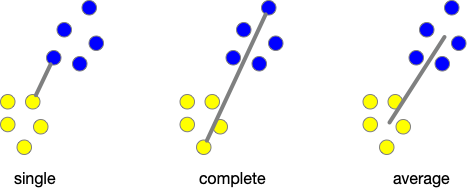
- average: $$d(u,v) = \sum_{ij}\frac{d(u_i,v_j)}{|u||v|}$$
- complete or farthest point: $$d(u,v) = \max(dist(u_i,v_j))$$
- single or nearest point: $$d(u,v) = \min(dist(u_i,v_j))$$
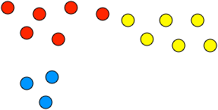
%%html

<img src="imgs/clusterpoints.png">
<div id="cluspts" style="width: 500px"></div>
<script>
$('head').append('<link rel="stylesheet" href="https://bits.csb.pitt.edu/asker.js/themes/asker.default.css" />');

    var divid = '#cluspts';
	jQuery(divid).asker({
	    id: divid,
	    question: "What cluster is closest to red by single linkage? complete?",
		answers: ['blue, blue','blue, yellow','yellow, blue','yellow, yellow'],
        server: "https://bits.csb.pitt.edu/asker.js/example/asker.cgi",
		charter: chartmaker})

$(".jp-InputArea .o:contains(html)").closest('.jp-InputArea').hide();


</script>
linkage
scipy.cluster.hierarchy.linkage creates a clustering hierarchy. It takes three parameters:
- y the data or a precalculated distance matrix
- method the linkage method (default single)
- metric the distance metric to use (default euclidean)
import scipy.cluster.hierarchy as hclust
linkage_matrix = hclust.linkage(randpts)
A (n−1) by 4 matrix Z is returned. At the i-th iteration, clusters with indices Z[i, 0] and Z[i, 1] are combined to form cluster n+i. A cluster with an index less than n corresponds to one of the n original observations. The distance between clusters Z[i, 0] and Z[i, 1] is given by Z[i, 2]. The fourth value Z[i, 3] represents the number of original observations in the newly formed cluster.linkage_matrix.shape
(199, 4)
linkage_matrix
array([[1.49000000e+02, 1.71000000e+02, 4.46097932e-03, 2.00000000e+00],
       [4.60000000e+01, 7.20000000e+01, 6.85261819e-03, 2.00000000e+00],
       [1.60000000e+01, 7.30000000e+01, 1.51521318e-02, 2.00000000e+00],
       [1.37000000e+02, 1.57000000e+02, 1.53148351e-02, 2.00000000e+00],
       [1.19000000e+02, 1.89000000e+02, 1.78213509e-02, 2.00000000e+00],
       [1.22000000e+02, 1.98000000e+02, 2.04763202e-02, 2.00000000e+00],
       [1.34000000e+02, 2.00000000e+02, 2.35915430e-02, 3.00000000e+00],
       [1.38000000e+02, 1.87000000e+02, 2.65878878e-02, 2.00000000e+00],
       [2.40000000e+01, 6.90000000e+01, 2.93336673e-02, 2.00000000e+00],
       [6.00000000e+01, 9.60000000e+01, 2.99804179e-02, 2.00000000e+00],
       [1.82000000e+02, 1.85000000e+02, 3.14543289e-02, 2.00000000e+00],
       [1.54000000e+02, 1.96000000e+02, 3.38672911e-02, 2.00000000e+00],
       [9.00000000e+00, 1.76000000e+02, 3.54702089e-02, 2.00000000e+00],
       [3.90000000e+01, 2.12000000e+02, 3.56342391e-02, 3.00000000e+00],
       [2.03000000e+02, 2.09000000e+02, 3.78817319e-02, 4.00000000e+00],
       [1.15000000e+02, 1.47000000e+02, 4.09620150e-02, 2.00000000e+00],
       [3.00000000e+00, 1.74000000e+02, 4.09881290e-02, 2.00000000e+00],
       [6.00000000e+00, 9.90000000e+01, 4.14929659e-02, 2.00000000e+00],
       [9.00000000e+01, 1.72000000e+02, 4.16513026e-02, 2.00000000e+00],
       [1.40000000e+01, 7.60000000e+01, 4.26578945e-02, 2.00000000e+00],
       [1.30000000e+01, 4.10000000e+01, 4.30331868e-02, 2.00000000e+00],
       [1.27000000e+02, 2.15000000e+02, 4.37628602e-02, 3.00000000e+00],
       [1.36000000e+02, 1.64000000e+02, 4.38642461e-02, 2.00000000e+00],
       [6.20000000e+01, 2.13000000e+02, 4.46924715e-02, 4.00000000e+00],
       [1.68000000e+02, 1.91000000e+02, 4.64564965e-02, 2.00000000e+00],
       [1.35000000e+02, 1.41000000e+02, 4.71929887e-02, 2.00000000e+00],
       [8.70000000e+01, 2.16000000e+02, 4.78129247e-02, 3.00000000e+00],
       [1.53000000e+02, 2.02000000e+02, 4.80458906e-02, 3.00000000e+00],
       [5.80000000e+01, 7.50000000e+01, 4.90392524e-02, 2.00000000e+00],
       [2.00000000e+01, 2.26000000e+02, 5.04661397e-02, 4.00000000e+00],
       [2.00000000e+00, 2.29000000e+02, 5.12219112e-02, 5.00000000e+00],
       [2.70000000e+01, 1.56000000e+02, 5.27747011e-02, 2.00000000e+00],
       [4.00000000e+00, 2.01000000e+02, 5.40595777e-02, 3.00000000e+00],
       [3.10000000e+01, 5.50000000e+01, 5.53762069e-02, 2.00000000e+00],
       [8.00000000e+00, 1.94000000e+02, 5.62458425e-02, 2.00000000e+00],
       [5.00000000e+01, 1.88000000e+02, 5.65509970e-02, 2.00000000e+00],
       [1.50000000e+01, 2.30000000e+02, 5.71721638e-02, 6.00000000e+00],
       [2.14000000e+02, 2.28000000e+02, 5.76827887e-02, 6.00000000e+00],
       [4.70000000e+01, 5.20000000e+01, 5.78110419e-02, 2.00000000e+00],
       [3.50000000e+01, 9.40000000e+01, 5.82658131e-02, 2.00000000e+00],
       [2.32000000e+02, 2.39000000e+02, 5.86789916e-02, 5.00000000e+00],
       [1.62000000e+02, 1.83000000e+02, 5.86848206e-02, 2.00000000e+00],
       [1.70000000e+02, 1.77000000e+02, 5.86978283e-02, 2.00000000e+00],
       [1.80000000e+01, 2.17000000e+02, 5.91950496e-02, 3.00000000e+00],
       [8.20000000e+01, 2.19000000e+02, 6.11521167e-02, 3.00000000e+00],
       [3.70000000e+01, 2.23000000e+02, 6.12666247e-02, 5.00000000e+00],
       [4.80000000e+01, 5.90000000e+01, 6.28201204e-02, 2.00000000e+00],
       [1.07000000e+02, 2.10000000e+02, 6.35916605e-02, 3.00000000e+00],
       [3.40000000e+01, 2.27000000e+02, 6.37643821e-02, 4.00000000e+00],
       [1.25000000e+02, 1.84000000e+02, 6.38771083e-02, 2.00000000e+00],
       [1.20000000e+02, 2.34000000e+02, 6.75200732e-02, 3.00000000e+00],
       [5.10000000e+01, 2.38000000e+02, 6.75869041e-02, 3.00000000e+00],
       [1.29000000e+02, 2.42000000e+02, 6.80689763e-02, 3.00000000e+00],
       [2.80000000e+01, 3.30000000e+01, 6.84683645e-02, 2.00000000e+00],
       [6.30000000e+01, 2.44000000e+02, 6.84799076e-02, 4.00000000e+00],
       [7.10000000e+01, 2.45000000e+02, 7.08571666e-02, 6.00000000e+00],
       [1.03000000e+02, 1.23000000e+02, 7.10883173e-02, 2.00000000e+00],
       [2.48000000e+02, 2.55000000e+02, 7.16967897e-02, 1.00000000e+01],
       [2.20000000e+01, 1.00000000e+02, 7.24315337e-02, 2.00000000e+00],
       [1.16000000e+02, 2.04000000e+02, 7.24882884e-02, 3.00000000e+00],
       [1.55000000e+02, 2.50000000e+02, 7.27899910e-02, 4.00000000e+00],
       [1.30000000e+02, 1.31000000e+02, 7.44755175e-02, 2.00000000e+00],
       [2.11000000e+02, 2.41000000e+02, 7.49720297e-02, 4.00000000e+00],
       [8.00000000e+01, 2.57000000e+02, 7.53968749e-02, 1.10000000e+01],
       [1.92000000e+02, 2.24000000e+02, 7.75842496e-02, 3.00000000e+00],
       [1.26000000e+02, 1.51000000e+02, 7.84050402e-02, 2.00000000e+00],
       [5.70000000e+01, 2.40000000e+02, 7.84796537e-02, 6.00000000e+00],
       [2.58000000e+02, 2.60000000e+02, 7.89227377e-02, 6.00000000e+00],
       [1.66000000e+02, 1.79000000e+02, 7.94677176e-02, 2.00000000e+00],
       [2.54000000e+02, 2.63000000e+02, 8.15415392e-02, 1.50000000e+01],
       [5.60000000e+01, 6.50000000e+01, 8.20849532e-02, 2.00000000e+00],
       [2.52000000e+02, 2.56000000e+02, 8.33896565e-02, 5.00000000e+00],
       [1.80000000e+02, 2.25000000e+02, 8.43081124e-02, 3.00000000e+00],
       [2.33000000e+02, 2.37000000e+02, 8.44501404e-02, 8.00000000e+00],
       [2.49000000e+02, 2.64000000e+02, 8.50561984e-02, 5.00000000e+00],
       [7.00000000e+01, 2.73000000e+02, 8.54845459e-02, 9.00000000e+00],
       [1.14000000e+02, 2.65000000e+02, 8.63919637e-02, 3.00000000e+00],
       [2.05000000e+02, 2.67000000e+02, 8.65156493e-02, 8.00000000e+00],
       [1.90000000e+01, 1.95000000e+02, 8.88527318e-02, 2.00000000e+00],
       [1.46000000e+02, 2.68000000e+02, 8.90563045e-02, 3.00000000e+00],
       [8.50000000e+01, 9.70000000e+01, 8.93399421e-02, 2.00000000e+00],
       [0.00000000e+00, 2.90000000e+01, 9.00439497e-02, 2.00000000e+00],
       [1.69000000e+02, 2.76000000e+02, 9.04181689e-02, 4.00000000e+00],
       [2.61000000e+02, 2.69000000e+02, 9.15308412e-02, 1.70000000e+01],
       [1.81000000e+02, 2.71000000e+02, 9.24404679e-02, 6.00000000e+00],
       [1.10000000e+02, 2.62000000e+02, 9.24512863e-02, 5.00000000e+00],
       [2.06000000e+02, 2.59000000e+02, 9.28490269e-02, 6.00000000e+00],
       [2.21000000e+02, 2.85000000e+02, 9.33121189e-02, 8.00000000e+00],
       [2.10000000e+01, 2.80000000e+02, 9.33449228e-02, 3.00000000e+00],
       [2.46000000e+02, 2.75000000e+02, 9.44668630e-02, 1.10000000e+01],
       [9.20000000e+01, 2.81000000e+02, 9.82526818e-02, 3.00000000e+00],
       [3.20000000e+01, 8.90000000e+01, 9.83514763e-02, 2.00000000e+00],
       [2.66000000e+02, 2.78000000e+02, 9.92969524e-02, 8.00000000e+00],
       [1.70000000e+01, 2.83000000e+02, 1.00235834e-01, 1.80000000e+01],
       [2.50000000e+01, 9.50000000e+01, 1.01665792e-01, 2.00000000e+00],
       [1.86000000e+02, 2.36000000e+02, 1.07180172e-01, 7.00000000e+00],
       [9.80000000e+01, 2.90000000e+02, 1.07841537e-01, 4.00000000e+00],
       [4.00000000e+01, 6.10000000e+01, 1.08468612e-01, 2.00000000e+00],
       [2.74000000e+02, 2.82000000e+02, 1.09930262e-01, 9.00000000e+00],
       [1.04000000e+02, 1.99000000e+02, 1.10531529e-01, 2.00000000e+00],
       [2.77000000e+02, 2.98000000e+02, 1.13211503e-01, 1.70000000e+01],
       [2.07000000e+02, 3.00000000e+02, 1.13522406e-01, 1.90000000e+01],
       [8.30000000e+01, 3.01000000e+02, 1.14183848e-01, 2.00000000e+01],
       [1.00000000e+00, 1.18000000e+02, 1.15628703e-01, 2.00000000e+00],
       [1.33000000e+02, 1.59000000e+02, 1.15690794e-01, 2.00000000e+00],
       [2.88000000e+02, 2.96000000e+02, 1.16741096e-01, 7.00000000e+00],
       [5.40000000e+01, 2.35000000e+02, 1.18258150e-01, 3.00000000e+00],
       [7.70000000e+01, 9.10000000e+01, 1.18371150e-01, 2.00000000e+00],
       [3.00000000e+01, 2.20000000e+02, 1.18453723e-01, 3.00000000e+00],
       [1.11000000e+02, 1.63000000e+02, 1.18467821e-01, 2.00000000e+00],
       [1.08000000e+02, 1.58000000e+02, 1.18605371e-01, 2.00000000e+00],
       [2.89000000e+02, 3.06000000e+02, 1.20369073e-01, 1.40000000e+01],
       [1.12000000e+02, 2.84000000e+02, 1.20939623e-01, 7.00000000e+00],
       [2.31000000e+02, 2.95000000e+02, 1.21421162e-01, 9.00000000e+00],
       [2.92000000e+02, 3.11000000e+02, 1.21908215e-01, 2.20000000e+01],
       [2.30000000e+01, 3.60000000e+01, 1.24742435e-01, 2.00000000e+00],
       [1.00000000e+01, 7.40000000e+01, 1.25836946e-01, 2.00000000e+00],
       [2.93000000e+02, 3.14000000e+02, 1.27005757e-01, 4.00000000e+01],
       [1.40000000e+02, 3.17000000e+02, 1.27480221e-01, 4.10000000e+01],
       [1.61000000e+02, 2.79000000e+02, 1.28443916e-01, 4.00000000e+00],
       [2.18000000e+02, 3.18000000e+02, 1.30309737e-01, 4.30000000e+01],
       [3.13000000e+02, 3.20000000e+02, 1.30499868e-01, 5.20000000e+01],
       [3.05000000e+02, 3.21000000e+02, 1.31250675e-01, 5.90000000e+01],
       [3.07000000e+02, 3.15000000e+02, 1.32289231e-01, 4.00000000e+00],
       [2.43000000e+02, 2.94000000e+02, 1.32325830e-01, 5.00000000e+00],
       [3.09000000e+02, 3.12000000e+02, 1.32484499e-01, 9.00000000e+00],
       [3.03000000e+02, 3.22000000e+02, 1.33829293e-01, 6.10000000e+01],
       [1.67000000e+02, 2.22000000e+02, 1.34803524e-01, 3.00000000e+00],
       [1.02000000e+02, 3.04000000e+02, 1.36009814e-01, 3.00000000e+00],
       [1.13000000e+02, 1.78000000e+02, 1.37101208e-01, 2.00000000e+00],
       [4.40000000e+01, 8.10000000e+01, 1.37338461e-01, 2.00000000e+00],
       [7.90000000e+01, 3.08000000e+02, 1.37668275e-01, 4.00000000e+00],
       [1.24000000e+02, 3.19000000e+02, 1.38750896e-01, 5.00000000e+00],
       [3.02000000e+02, 3.26000000e+02, 1.40738695e-01, 8.10000000e+01],
       [2.08000000e+02, 2.53000000e+02, 1.40804349e-01, 4.00000000e+00],
       [3.80000000e+01, 3.33000000e+02, 1.41390485e-01, 8.20000000e+01],
       [4.90000000e+01, 3.31000000e+02, 1.42777393e-01, 5.00000000e+00],
       [3.25000000e+02, 3.32000000e+02, 1.42966246e-01, 1.40000000e+01],
       [1.10000000e+01, 3.30000000e+02, 1.43558272e-01, 3.00000000e+00],
       [8.40000000e+01, 3.35000000e+02, 1.49205129e-01, 8.30000000e+01],
       [1.21000000e+02, 3.39000000e+02, 1.50857936e-01, 8.40000000e+01],
       [2.87000000e+02, 3.40000000e+02, 1.53037165e-01, 9.20000000e+01],
       [2.60000000e+01, 3.41000000e+02, 1.53058594e-01, 9.30000000e+01],
       [6.40000000e+01, 3.42000000e+02, 1.53485686e-01, 9.40000000e+01],
       [2.51000000e+02, 3.34000000e+02, 1.55617162e-01, 7.00000000e+00],
       [1.93000000e+02, 3.43000000e+02, 1.55680672e-01, 9.50000000e+01],
       [1.60000000e+02, 3.45000000e+02, 1.57148964e-01, 9.60000000e+01],
       [3.24000000e+02, 3.46000000e+02, 1.57829263e-01, 1.01000000e+02],
       [4.20000000e+01, 3.16000000e+02, 1.59739095e-01, 3.00000000e+00],
       [3.27000000e+02, 3.29000000e+02, 1.62354589e-01, 5.00000000e+00],
       [3.37000000e+02, 3.49000000e+02, 1.62365869e-01, 1.90000000e+01],
       [1.52000000e+02, 1.65000000e+02, 1.62771714e-01, 2.00000000e+00],
       [1.06000000e+02, 3.50000000e+02, 1.64820991e-01, 2.00000000e+01],
       [3.28000000e+02, 3.47000000e+02, 1.66258090e-01, 1.04000000e+02],
       [3.23000000e+02, 3.53000000e+02, 1.66872701e-01, 1.08000000e+02],
       [3.44000000e+02, 3.54000000e+02, 1.67675789e-01, 1.15000000e+02],
       [2.72000000e+02, 2.91000000e+02, 1.70312886e-01, 5.00000000e+00],
       [1.05000000e+02, 3.51000000e+02, 1.70622544e-01, 3.00000000e+00],
       [1.17000000e+02, 1.44000000e+02, 1.73703505e-01, 2.00000000e+00],
       [1.43000000e+02, 3.52000000e+02, 1.74719291e-01, 2.10000000e+01],
       [7.00000000e+00, 3.55000000e+02, 1.75831645e-01, 1.16000000e+02],
       [1.28000000e+02, 3.60000000e+02, 1.80161169e-01, 1.17000000e+02],
       [3.48000000e+02, 3.61000000e+02, 1.82127024e-01, 1.20000000e+02],
       [1.48000000e+02, 2.99000000e+02, 1.86143420e-01, 3.00000000e+00],
       [3.56000000e+02, 3.62000000e+02, 1.89421685e-01, 1.25000000e+02],
       [2.70000000e+02, 3.64000000e+02, 1.96936021e-01, 1.27000000e+02],
       [1.75000000e+02, 3.59000000e+02, 1.96974837e-01, 2.20000000e+01],
       [1.20000000e+01, 4.30000000e+01, 1.97920845e-01, 2.00000000e+00],
       [2.97000000e+02, 3.36000000e+02, 2.00391424e-01, 7.00000000e+00],
       [1.39000000e+02, 3.65000000e+02, 2.01299338e-01, 1.28000000e+02],
       [6.70000000e+01, 3.67000000e+02, 2.04332642e-01, 3.00000000e+00],
       [2.86000000e+02, 3.66000000e+02, 2.12902916e-01, 2.80000000e+01],
       [3.69000000e+02, 3.71000000e+02, 2.13142279e-01, 1.56000000e+02],
       [1.32000000e+02, 3.72000000e+02, 2.18065620e-01, 1.57000000e+02],
       [1.42000000e+02, 3.73000000e+02, 2.18451186e-01, 1.58000000e+02],
       [3.58000000e+02, 3.74000000e+02, 2.18791278e-01, 1.60000000e+02],
       [3.57000000e+02, 3.75000000e+02, 2.21760753e-01, 1.63000000e+02],
       [1.01000000e+02, 3.76000000e+02, 2.35723986e-01, 1.64000000e+02],
       [3.63000000e+02, 3.77000000e+02, 2.43024267e-01, 1.67000000e+02],
       [5.00000000e+00, 3.68000000e+02, 2.44111723e-01, 8.00000000e+00],
       [1.90000000e+02, 3.78000000e+02, 2.44400296e-01, 1.68000000e+02],
       [2.47000000e+02, 3.80000000e+02, 2.46223922e-01, 1.71000000e+02],
       [5.30000000e+01, 3.79000000e+02, 2.50725745e-01, 9.00000000e+00],
       [1.97000000e+02, 3.81000000e+02, 2.54748265e-01, 1.72000000e+02],
       [7.80000000e+01, 3.83000000e+02, 2.55507470e-01, 1.73000000e+02],
       [3.38000000e+02, 3.84000000e+02, 2.61522515e-01, 1.76000000e+02],
       [3.70000000e+02, 3.82000000e+02, 3.00532955e-01, 1.20000000e+01],
       [3.10000000e+02, 3.85000000e+02, 3.14559328e-01, 1.78000000e+02],
       [4.50000000e+01, 3.87000000e+02, 3.26139012e-01, 1.79000000e+02],
       [6.80000000e+01, 3.88000000e+02, 3.95954374e-01, 1.80000000e+02],
       [3.86000000e+02, 3.89000000e+02, 3.98516147e-01, 1.92000000e+02],
       [1.73000000e+02, 3.90000000e+02, 4.15355443e-01, 1.93000000e+02],
       [1.09000000e+02, 1.50000000e+02, 4.41810997e-01, 2.00000000e+00],
       [6.60000000e+01, 3.91000000e+02, 5.56731638e-01, 1.94000000e+02],
       [1.45000000e+02, 3.92000000e+02, 7.08316589e-01, 3.00000000e+00],
       [3.93000000e+02, 3.94000000e+02, 7.69909958e-01, 1.97000000e+02],
       [8.80000000e+01, 9.30000000e+01, 8.46319094e-01, 2.00000000e+00],
       [8.60000000e+01, 3.95000000e+02, 8.79918242e-01, 1.98000000e+02],
       [3.96000000e+02, 3.97000000e+02, 9.84658940e-01, 2.00000000e+02]])
Dendograms
hclust.dendrogram(linkage_matrix,p=10,truncate_mode='level',no_labels=True);#show first 10 levels

The cophenetic distance between two observations that have been clustered is defined to be the intergroup dissimilarity at which the two observations are first combined into a single cluster. It is shown as the height of the U-links.
fcluster: extracting clusters from a hierarchy
fcluster takes a linkage matrix and returns a cluster assignment. It takes a threshold value and a string specifying what method to use to form the cluster.
help(hclust.fcluster)
Help on function fcluster in module scipy.cluster.hierarchy:

fcluster(Z, t, criterion='inconsistent', depth=2, R=None, monocrit=None)
    Form flat clusters from the hierarchical clustering defined by
    the given linkage matrix.

    Parameters
    ----------
    Z : ndarray
        The hierarchical clustering encoded with the matrix returned
        by the `linkage` function.
    t : scalar
        For criteria 'inconsistent', 'distance' or 'monocrit',
         this is the threshold to apply when forming flat clusters.
        For 'maxclust' or 'maxclust_monocrit' criteria,
         this would be max number of clusters requested.
    criterion : str, optional
        The criterion to use in forming flat clusters. This can
        be any of the following values:

          ``inconsistent`` :
              If a cluster node and all its
              descendants have an inconsistent value less than or equal
              to `t`, then all its leaf descendants belong to the
              same flat cluster. When no non-singleton cluster meets
              this criterion, every node is assigned to its own
              cluster. (Default)

          ``distance`` :
              Forms flat clusters so that the original
              observations in each flat cluster have no greater a
              cophenetic distance than `t`.

          ``maxclust`` :
              Finds a minimum threshold ``r`` so that
              the cophenetic distance between any two original
              observations in the same flat cluster is no more than
              ``r`` and no more than `t` flat clusters are formed.

          ``monocrit`` :
              Forms a flat cluster from a cluster node c
              with index i when ``monocrit[j] <= t``.

              For example, to threshold on the maximum mean distance
              as computed in the inconsistency matrix R with a
              threshold of 0.8 do::

                  MR = maxRstat(Z, R, 3)
                  fcluster(Z, t=0.8, criterion='monocrit', monocrit=MR)

          ``maxclust_monocrit`` :
              Forms a flat cluster from a
              non-singleton cluster node ``c`` when ``monocrit[i] <=
              r`` for all cluster indices ``i`` below and including
              ``c``. ``r`` is minimized such that no more than ``t``
              flat clusters are formed. monocrit must be
              monotonic. For example, to minimize the threshold t on
              maximum inconsistency values so that no more than 3 flat
              clusters are formed, do::

                  MI = maxinconsts(Z, R)
                  fcluster(Z, t=3, criterion='maxclust_monocrit', monocrit=MI)
    depth : int, optional
        The maximum depth to perform the inconsistency calculation.
        It has no meaning for the other criteria. Default is 2.
    R : ndarray, optional
        The inconsistency matrix to use for the 'inconsistent'
        criterion. This matrix is computed if not provided.
    monocrit : ndarray, optional
        An array of length n-1. `monocrit[i]` is the
        statistics upon which non-singleton i is thresholded. The
        monocrit vector must be monotonic, i.e., given a node c with
        index i, for all node indices j corresponding to nodes
        below c, ``monocrit[i] >= monocrit[j]``.

    Returns
    -------
    fcluster : ndarray
        An array of length ``n``. ``T[i]`` is the flat cluster number to
        which original observation ``i`` belongs.

    See Also
    --------
    linkage : for information about hierarchical clustering methods work.

    Examples
    --------
    >>> from scipy.cluster.hierarchy import ward, fcluster
    >>> from scipy.spatial.distance import pdist

    All cluster linkage methods - e.g., `scipy.cluster.hierarchy.ward`
    generate a linkage matrix ``Z`` as their output:

    >>> X = [[0, 0], [0, 1], [1, 0],
    ...      [0, 4], [0, 3], [1, 4],
    ...      [4, 0], [3, 0], [4, 1],
    ...      [4, 4], [3, 4], [4, 3]]

    >>> Z = ward(pdist(X))

    >>> Z
    array([[ 0.        ,  1.        ,  1.        ,  2.        ],
           [ 3.        ,  4.        ,  1.        ,  2.        ],
           [ 6.        ,  7.        ,  1.        ,  2.        ],
           [ 9.        , 10.        ,  1.        ,  2.        ],
           [ 2.        , 12.        ,  1.29099445,  3.        ],
           [ 5.        , 13.        ,  1.29099445,  3.        ],
           [ 8.        , 14.        ,  1.29099445,  3.        ],
           [11.        , 15.        ,  1.29099445,  3.        ],
           [16.        , 17.        ,  5.77350269,  6.        ],
           [18.        , 19.        ,  5.77350269,  6.        ],
           [20.        , 21.        ,  8.16496581, 12.        ]])

    This matrix represents a dendrogram, where the first and second elements
    are the two clusters merged at each step, the third element is the
    distance between these clusters, and the fourth element is the size of
    the new cluster - the number of original data points included.

    `scipy.cluster.hierarchy.fcluster` can be used to flatten the
    dendrogram, obtaining as a result an assignation of the original data
    points to single clusters.

    This assignation mostly depends on a distance threshold ``t`` - the maximum
    inter-cluster distance allowed:

    >>> fcluster(Z, t=0.9, criterion='distance')
    array([ 1,  2,  3,  4,  5,  6,  7,  8,  9, 10, 11, 12], dtype=int32)

    >>> fcluster(Z, t=1.1, criterion='distance')
    array([1, 1, 2, 3, 3, 4, 5, 5, 6, 7, 7, 8], dtype=int32)

    >>> fcluster(Z, t=3, criterion='distance')
    array([1, 1, 1, 2, 2, 2, 3, 3, 3, 4, 4, 4], dtype=int32)

    >>> fcluster(Z, t=9, criterion='distance')
    array([1, 1, 1, 1, 1, 1, 1, 1, 1, 1, 1, 1], dtype=int32)

    In the first case, the threshold ``t`` is too small to allow any two
    samples in the data to form a cluster, so 12 different clusters are
    returned.

    In the second case, the threshold is large enough to allow the first
    4 points to be merged with their nearest neighbors. So, here, only 8
    clusters are returned.

    The third case, with a much higher threshold, allows for up to 8 data
    points to be connected - so 4 clusters are returned here.

    Lastly, the threshold of the fourth case is large enough to allow for
    all data points to be merged together - so a single cluster is returned.
Flatten based on distance threshold
clusters = hclust.fcluster(linkage_matrix,0.3,'distance')
len(set(clusters))
14
plt.scatter(randpts[:,0],randpts[:,1],c=clusters);

Flatten based on number of clusters
clusters = hclust.fcluster(linkage_matrix,4,'maxclust')
len(set(clusters))
4
plt.scatter(randpts[:,0],randpts[:,1],c=clusters)
<matplotlib.collections.PathCollection at 0x135996b4550>

fclusterdata
fclusterdata does both linkage and fcluster in one step. Let's try out different linkage methods.
clusters = hclust.fclusterdata(randpts,.3,criterion='distance',method='single')
plt.scatter(randpts[:,0],randpts[:,1],c=clusters)
len(set(clusters))
14
clusters = hclust.fclusterdata(randpts,.3,criterion='distance',method='complete')
plt.scatter(randpts[:,0],randpts[:,1],c=clusters);
len(set(clusters))
63

clusters = hclust.fclusterdata(randpts,4,'maxclust',method='complete')
plt.scatter(randpts[:,0],randpts[:,1],c=clusters);

clusters = hclust.fclusterdata(randpts,4,'maxclust',method='average')
plt.scatter(randpts[:,0],randpts[:,1],c=clusters);

You can even use a non-Euclidean metric.
clusters = hclust.fclusterdata(randpts,4,'maxclust',method='complete',metric='cityblock')
plt.scatter(randpts[:,0],randpts[:,1],c=clusters);

%%html

<img src="imgs/roll.png">
<div id="clusroll" style="width: 500px"></div>
<script>
$('head').append('<link rel="stylesheet" href="https://bits.csb.pitt.edu/asker.js/themes/asker.default.css" />');

    var divid = '#clusroll';
	jQuery(divid).asker({
	    id: divid,
	    question: "What linkage was likely used to form these clusters?",
		answers: ['average','complete','single'],
        server: "https://bits.csb.pitt.edu/asker.js/example/asker.cgi",
		charter: chartmaker})

$(".jp-InputArea .o:contains(html)").closest('.jp-InputArea').hide();


</script>
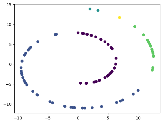
leaves_list
A hierarchical cluster imposes an order on the leaves. You can retrieve this ordering from the linkage matrix with leaves_list
hclust.leaves_list(linkage_matrix)
array([ 88,  93,  86,  66, 173,  67,  12,  43,  53,   5,  40,  61,  49,
        79,  30,  13,  41,  68,  45, 108, 158,  11,  44,  81,  78, 197,
       107, 182, 185, 190, 148, 104, 199, 101, 105, 152, 165, 117, 144,
       142, 132, 139,  56,  65, 180, 135, 141,  32,  89,  42,  10,  74,
       128,   7,  51,  47,  52,  24,  69,  28,  33,  77,  91,  23,  36,
       102, 133, 159,  18,   6,  99,  25,  95, 160, 193,  64,  26, 127,
       115, 147, 110, 154, 196, 162, 183, 121,  84,  38,  83, 138, 187,
       122, 198,  22, 100, 155, 120,   8, 194, 125, 184, 192, 168, 191,
       169, 114, 126, 151,   1, 118,  21,  85,  97,  98,  92,   0,  29,
        27, 156, 186,  15,   2,  20,  87,   3, 174,  90, 172, 140,  17,
       130, 131,  63,  82,  14,  76,  80,  34, 153,  16,  73,  71,  37,
        62,  39,   9, 176,  57,   4,  46,  72,  35,  94,  19, 195,  48,
        59,  70,  31,  55, 137, 157,  60,  96,  58,  75,  54,  50, 188,
       134, 149, 171, 116, 119, 189, 175, 143, 106, 111, 163, 112, 181,
       129, 170, 177, 103, 123, 124, 161, 146, 166, 179, 167, 136, 164,
       113, 178, 145, 109, 150], dtype=int32)
plt.figure(figsize=(16,3))
hclust.dendrogram(linkage_matrix);

%%html
<div id="listorder" style="width: 500px"></div>
<script>
$('head').append('<link rel="stylesheet" href="https://bits.csb.pitt.edu/asker.js/themes/asker.default.css" />');

    var divid = '#listorder';
	jQuery(divid).asker({
	    id: divid,
	    question: "Is this order unique for a given linkage matrix?",
		answers: ['Yes','No'],
        server: "https://bits.csb.pitt.edu/asker.js/example/asker.cgi",
		charter: chartmaker})

$(".jp-InputArea .o:contains(html)").closest('.jp-InputArea').hide();


</script>
Project: Cluster Expression Data
- Download https://asinansaglam.github.io/python_bio_2022/files/Spellman.csv
- read the expression data into a numpy array (hint:
np.genfromtxt) - cluster it with the default parameters
- retrieve the leaves
- reorder the orginal data according the the leaf order
- display the result as a heatmap (
plt.matshow) - try different distance metrics and linkages - what gives the best result?
!wget https://asinansaglam.github.io/python_bio_2022/files/Spellman.csv
--2023-10-16 16:47:44--  https://asinansaglam.github.io/python_bio_2022/files/Spellman.csv
Resolving asinansaglam.github.io (asinansaglam.github.io)... 185.199.108.153, 185.199.109.153, 185.199.110.153, ...
Connecting to asinansaglam.github.io (asinansaglam.github.io)|185.199.108.153|:443... connected.
HTTP request sent, awaiting response... 200 OK
Length: 609183 (595K) [text/csv]
Saving to: 'Spellman.csv.3'

     0K .......... .......... .......... .......... ..........  8% 9.22M 0s
    50K .......... .......... .......... .......... .......... 16% 20.2M 0s
   100K .......... .......... .......... .......... .......... 25% 16.4M 0s
   150K .......... .......... .......... .......... .......... 33% 20.8M 0s
   200K .......... .......... .......... .......... .......... 42% 64.9M 0s
   250K .......... .......... .......... .......... .......... 50% 16.4M 0s
   300K .......... .......... .......... .......... .......... 58% 55.0M 0s
   350K .......... .......... .......... .......... .......... 67% 65.5M 0s
   400K .......... .......... .......... .......... .......... 75% 8.90M 0s
   450K .......... .......... .......... .......... .......... 84%  157M 0s
   500K .......... .......... .......... .......... .......... 92%  139M 0s
   550K .......... .......... .......... .......... ....      100%  194M=0.02s

2023-10-16 16:47:44 (23.5 MB/s) - 'Spellman.csv.3' saved [609183/609183]
from matplotlib.pylab import cm
import numpy as np
import scipy.cluster.hierarchy as hclust
import matplotlib.pyplot as plt
data = np.genfromtxt('Spellman.csv',skip_header=1,delimiter=',')[:,1:]
Z = hclust.linkage(data,method='complete')
leaves = hclust.leaves_list(Z)
ordered = data[leaves]
plt.matshow(ordered,aspect=0.01,cmap=cm.seismic);

plt.matshow(data,aspect=0.01,cmap=cm.seismic);
