Dictionary
A dictionary is an unordered collection of key,value pairs where the keys are mapped to values.
A dictionary object is indexed by the key to get the value.
d = dict()
d['key'] = 'value'
d[0] = ['x','y','z']
print(d)
{'key': 'value', 0: ['x', 'y', 'z']}
Initializing dicts
empty = dict()
alsoempty = {}
Specify key:value pairs within curly braces.
example = {'a': 1, 'b':2}
example
{'a': 1, 'b': 2}
Add new values by indexing with new/existing key
example['a'] = 0
example['z'] = 26
example
{'a': 0, 'b': 2, 'z': 26}
Accessing values
#example['c'] #keys must exist
Use in to test for membership
'c' in example
False
if 'c' not in example:
    example['c'] = 0
example
{'a': 0, 'b': 2, 'z': 26, 'c': 0}
Methods
example.keys()
dict_keys(['a', 'b', 'z', 'c'])
example.values()
dict_values([0, 2, 26, 0])
example.items()
dict_items([('a', 0), ('b', 2), ('z', 26), ('c', 0)])
def count(vals):
    cnts = {}
    for x in vals:
        cnts[x] += 1
    return cnts
#d = count(['a','a','b','a','c','b'])
%%html
<div id="dictdefault" style="width: 500px"></div>
<script>
$('head').append('<link rel="stylesheet" href="http://bits.csb.pitt.edu/asker.js/themes/asker.default.css" />');

    var divid = '#dictdefault';
	jQuery(divid).asker({
	    id: divid,
	    question: "What is the value of <tt>d['a']</tt>?",
		answers: ["0","1","2","3","6",'Error'],
        server: "http://bits.csb.pitt.edu/asker.js/example/asker.cgi",
		charter: chartmaker})

$(".jp-InputArea .o:contains(html)").closest('.jp-InputArea').hide();


</script>
The Fix
def count(vals):
    cnts = {}
    for x in vals:
        if x not in cnts:
            cnts[x] = 0
        cnts[x] += 1
    return cnts

d = count(['a','a','b','a','c','b'])
d['a']
3
If this seems annoying, checkout collections.defaultdict
Sets
A set is an unordered collection with no duplicate elements. Basic uses include membership testing and eliminating duplicate entries. Set objects also support mathematical operations like union, intersection, difference, and symmetric difference.
Can initialize with a list
stuff = set(['a','b','a','d','x','a','e'])
stuff
{'a', 'b', 'd', 'e', 'x'}
Sets are not indexed - use add to insert new elements.
stuff.add('y')
set operations
Efficient membership testing
'y' in stuff
True
stuff2 = set(['a','b','c'])
print('and',stuff & stuff2) #intersection
and {'b', 'a'}
print('or', stuff | stuff2)
or {'x', 'a', 'd', 'e', 'c', 'b', 'y'}
print('diff', stuff - stuff2)
diff {'x', 'e', 'y', 'd'}
s = set([1,2,2,3,3,3,4,4,4,4])
%%html
<div id="dictset" style="width: 500px"></div>
<script>
$('head').append('<link rel="stylesheet" href="http://bits.csb.pitt.edu/asker.js/themes/asker.default.css" />');

    var divid = '#dictset';
	jQuery(divid).asker({
	    id: divid,
	    question: "What is <tt>len(s)</tt>?",
		answers: ["0","1","3","4","9","10",'Error'],
        server: "http://bits.csb.pitt.edu/asker.js/example/asker.cgi",
		charter: chartmaker})

$(".jp-InputArea .o:contains(html)").closest('.jp-InputArea').hide();


</script>
a = set([1,2,2,3])
b = set([2,3,3,4])
c = a & b
%%html
<div id="setinter" style="width: 500px"></div>
<script>
$('head').append('<link rel="stylesheet" href="http://bits.csb.pitt.edu/asker.js/themes/asker.default.css" />');

    var divid = '#setinter';
	jQuery(divid).asker({
	    id: divid,
	    question: "What is <tt>c</tt>?",
		answers: ["{1,2,3,4}","{2,2,3,3}","{2,3}","{1,4}",'Error'],
        server: "http://bits.csb.pitt.edu/asker.js/example/asker.cgi",
		charter: chartmaker})

$(".jp-InputArea .o:contains(html)").closest('.jp-InputArea').hide();


</script>
Tuples
A tuple is an immutable list.
t = tuple([1,2,3])
t
(1, 2, 3)
Tuples are initialized the same way as lists, just with parentheses
t = ('x',0,3.0)
l = ['x',0,3.0]
t,l
(('x', 0, 3.0), ['x', 0, 3.0])
'%s %d' % ('hello',3) # second operand of string % operator is tuple
'hello 3'
t = ('x',0,3.0)
#t[2] += 1
%%html
<div id="dictimm" style="width: 500px"></div>
<script>
$('head').append('<link rel="stylesheet" href="http://bits.csb.pitt.edu/asker.js/themes/asker.default.css" />');

    var divid = '#dictimm';
	jQuery(divid).asker({
	    id: divid,
	    question: "What is the value of <tt>t[2]</tt>?",
		answers: ["0","1","3.0","4.0",'Error'],
        server: "http://bits.csb.pitt.edu/asker.js/example/asker.cgi",
		charter: chartmaker})

$(".jp-InputArea .o:contains(html)").closest('.jp-InputArea').hide();


</script>
Keys
The keys of a dictionary or set should be immutable. Examples of immutable types are numbers, strings, tuples (that contain only immutable objects) and frozensets.
example[(1,2)] = 'a'
#example[[1,2]] = 'a'
Dictionaries and sets efficiently store data based on the properties of the key - if the properties of the key can change, then the data structure is broken and the data is not where it should be.
Efficiency
Imagine we have two lists, l1 and l2, and we want do something with the items that are in common in both lists. Here we'll just count them.
def listcnt(l1, l2):
    cnt = 0
    for x in l1:
            if x in l2:
                cnt += 1
    return cnt
def setcnt(l1, l2):
    cnt = 0
    s1 = set(l1)
    s2 = set(l2)
    for x in s1:
            if x in s2:
                cnt += 1
    return cnt
These two functions generate the same answer if the lists have all distinct elements.
%%html
<div id="dictspeed" style="width: 500px"></div>
<script>
$('head').append('<link rel="stylesheet" href="http://bits.csb.pitt.edu/asker.js/themes/asker.default.css" />');

    var divid = '#dictspeed';
	jQuery(divid).asker({
	    id: divid,
	    question: "Which function is faster?",
		answers: ['listcnt, by a lot','listcnt, by a little','about the same','setcnt, by a little','setcnt, by a lot'],
        server: "http://bits.csb.pitt.edu/asker.js/example/asker.cgi",
		charter: chartmaker})

$(".jp-InputArea .o:contains(html)").closest('.jp-InputArea').hide();


</script>
import time
l1 = list(range(40000))
l2 = list(range(1000,10000))

t0 = time.time()
listcnt(l1,l2)
t1 = time.time()
setcnt(l1,l2)
t2 = time.time()
print("listcnt time: ",t1-t0,'\nsetcnt time:',t2-t1)
listcnt time:  1.6977856159210205
setcnt time: 0.0020287036895751953
Can you think of another way?
t0 = time.time()
len(set(l1) & set(l2))
t3 = time.time()
print("set intersection time:",t3-t0)
set intersection time: 0.0011761188507080078
Do not do membership testing on lists
- Lists are ordered by the programmer, which means Python must examine every element to determine (non)membership.
- Dictionaries and sets are unordered so Python can store the contents in a way that makes membership testing efficient (using hashing)
Hashing
The keys of sets and dictionaries must be hashable types. Technically, this means they define methods __eq__ (or __cmp__) and __hash__.
A hash function (__hash__) takes an arbitrary object and produces a number. Objects that are identical (according to __eq__ or __cmp__) must hash to the same hash value.
What does this get us?
Accessing an element of an array of elements in memory (random access...) is as simple as computing a memory address (base of array plus offset). This is great if our keys are a dense array of integers (then we have a lookup table).
Hash functions provide a way to quickly index into an array of data even when are keys are arbitray objects.
Hashing
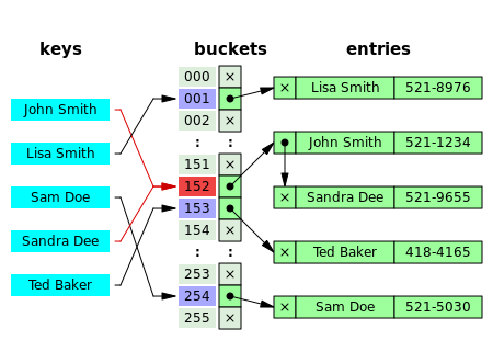
In this figure (from Wikipedia), collisions are resolved through chaining.
With a good hash function and enough buckets, no chain (list) will be more than a few elements long and accessing our data will be constant time (on average).
The position of an element in the table is determined by its hash value and the table size.
position = obj.__hash__() % table_size
Hash Functions
A good hash function of an object has the following properties:
- The hash value is fully determined by the object (deterministic).
- The hash function uses all the object's data (if relevant).
- The hash function is uniform (evenly distributes keys across the range)
The range of the hash function is usual the integers ($2^{32}$ or $2^{64}$).
print(hash(3), hash(1435080909832), hash('cat'), hash((3,'cat')))
3 1435080909832 -6816296582624972254 -746018197325947095
Implementing a Hash Function
You only need to implement a hash function when defining your own object types (which we haven't talked about yet...)
The best (and easiest) approach is to combine the built-in hash functions on your data.
a = 'cat'
b = 'dog'
print(hash(a))
print(hash(b))
print(hash( (a,b) ))
-6816296582624972254
1402495934381164085
4296283890760453472
Takeaway
sets, frozensets, and dicts use hashing to provide extremely efficient membership testing and (for dicts) value lookup.
However, you cannot rely on the order of data in these data structures. In fact, the order of items will change as you add and delete.
s = set([3,999])
s
{3, 999}
s.add(1000)
print(s)
s.update([1001,1002,1003])
{1000, 3, 999}
print(s)
{3, 999, 1000, 1001, 1002, 1003}
polyfit
Takes $x$ values, $y$ values, and degree of polynomial. Returns coefficients with least squares fit (highest degree first).
%%html
<div id="polydeg" style="width: 500px"></div>
<script>
$('head').append('<link rel="stylesheet" href="http://bits.csb.pitt.edu/asker.js/themes/asker.default.css" />');

    var divid = '#polydeg';
	jQuery(divid).asker({
	    id: divid,
	    question: "What degree is the polynomial 4x^2 + 5x - 3?",
		answers: ['1','2','3','4','5'],
        server: "http://bits.csb.pitt.edu/asker.js/example/asker.cgi",
		charter: chartmaker})

$(".jp-InputArea .o:contains(html)").closest('.jp-InputArea').hide();


</script>
import numpy as np
xvals = np.linspace(-1,2,20)
yvals = xvals**3 +np.random.random(20) #adds random numbers from 0 to 1 to 20 values of xvals
import matplotlib.pyplot as plt
%matplotlib inline
plt.plot(xvals,yvals,'o');

polyfit
deg1 = np.polyfit(xvals,yvals,1)
deg2 = np.polyfit(xvals,yvals,2)
deg3 = np.polyfit(xvals,yvals,3)
deg1
array([2.23836299, 0.6929211 ])
deg2
array([ 1.45320852, 0.78515446, -0.14841015])
%%html
<div id="deg3" style="width: 500px"></div>
<script>
$('head').append('<link rel="stylesheet" href="http://bits.csb.pitt.edu/asker.js/themes/asker.default.css" />');

    var divid = '#deg3';
	jQuery(divid).asker({
	    id: divid,
	    question: "What is the expected value of deg3[-1]?",
		answers: ['-1','0','0.5','1'],
        server: "http://bits.csb.pitt.edu/asker.js/example/asker.cgi",
		charter: chartmaker})

$(".jp-InputArea .o:contains(html)").closest('.jp-InputArea').hide();


</script>
%%html
<div id="deg3_2" style="width: 500px"></div>
<script>
$('head').append('<link rel="stylesheet" href="http://bits.csb.pitt.edu/asker.js/themes/asker.default.css" />');

    var divid = '#deg3_2';
	jQuery(divid).asker({
	    id: divid,
	    question: "What is the expected value of deg3[0]?",
		answers: ['-1','0','0.5','1'],
        server: "http://bits.csb.pitt.edu/asker.js/example/asker.cgi",
		charter: chartmaker})

$(".jp-InputArea .o:contains(html)").closest('.jp-InputArea').hide();


</script>
deg3
array([ 0.9782114 , -0.01410858, 0.06409614, 0.45667187])
deg3[-1]
0.4566718653971893
poly1d
Construct a polynomial function from coefficients
p1 = np.poly1d(deg1)
p2 = np.poly1d(deg2)
p3 = np.poly1d(deg3)
p1(2),p2(2),p3(2)
(5.169647076390596, 7.234732874955175, 8.354121049507011)
p1(0),p2(0),p3(0)
(0.6929211041311437, -0.14841014713590722, 0.4566718653971893)
plt.plot(xvals,yvals,'o',xvals,p1(xvals),'-',xvals,p2(xvals),'-',xvals,p3(xvals),'-');

scipy.optimize.curve_fit
Optimize fit to an arbitrary function. Returns optimal values (for least squares) of parameters along with covariance estimate.
Provide python function that takes x value and any parameters.
from scipy.optimize import curve_fit

def tanh(x,a,b):
    return b*np.tanh(a+x)

popt,pconv = curve_fit(tanh, xvals, yvals)
popt
array([0.30098577, 3.43896184])
plt.plot(xvals,yvals,'o',xvals,popt[1]*np.tanh(popt[0]+xvals)); plt.show()

Let's Analyze Data!
!wget https://asinansaglam.github.io/python_bio_2022/files/kd
!wget https://asinansaglam.github.io/python_bio_2022/files/aff.min
!wget https://asinansaglam.github.io/python_bio_2022/files/aff.score
--2022-09-20 01:29:33--  https://asinansaglam.github.io/python_bio_2022/files/kd
Resolving asinansaglam.github.io (asinansaglam.github.io)... 2606:50c0:8002::153, 2606:50c0:8003::153, 2606:50c0:8001::153, ...
Connecting to asinansaglam.github.io (asinansaglam.github.io)|2606:50c0:8002::153|:443... connected.
HTTP request sent, awaiting response... 200 OK
Length: 5262 (5.1K) [application/octet-stream]
Saving to: ‘kd.2’

kd.2                100%[===================>]   5.14K  --.-KB/s    in 0s

2022-09-20 01:29:33 (153 MB/s) - ‘kd.2’ saved [5262/5262]

--2022-09-20 01:29:33--  https://asinansaglam.github.io/python_bio_2022/files/aff.min
Resolving asinansaglam.github.io (asinansaglam.github.io)... 2606:50c0:8002::153, 2606:50c0:8003::153, 2606:50c0:8001::153, ...
Connecting to asinansaglam.github.io (asinansaglam.github.io)|2606:50c0:8002::153|:443... connected.
HTTP request sent, awaiting response... 200 OK
Length: 5678 (5.5K) [application/octet-stream]
Saving to: ‘aff.min.2’

aff.min.2           100%[===================>]   5.54K  --.-KB/s    in 0s

2022-09-20 01:29:34 (142 MB/s) - ‘aff.min.2’ saved [5678/5678]

--2022-09-20 01:29:34--  https://asinansaglam.github.io/python_bio_2022/files/aff.score
Resolving asinansaglam.github.io (asinansaglam.github.io)... 2606:50c0:8002::153, 2606:50c0:8003::153, 2606:50c0:8001::153, ...
Connecting to asinansaglam.github.io (asinansaglam.github.io)|2606:50c0:8002::153|:443... connected.
HTTP request sent, awaiting response... 200 OK
Length: 5659 (5.5K) [application/octet-stream]
Saving to: ‘aff.score.2’

aff.score.2         100%[===================>]   5.53K  --.-KB/s    in 0s

2022-09-20 01:29:34 (152 MB/s) - ‘aff.score.2’ saved [5659/5659]
!head kd
set1_1  3.34
set1_100  6.3
set1_102  8.62
set1_103  6.44
set1_104  -0.15
set1_105  8.48
set1_106  7.01
set1_107  4.61
set1_108  7.55
set1_109  7.96
kd contains experimental values while aff.min and aff.score contain computational predictions of the experimental values. Each line has a name and value.
How good are the predictions?
How do we want to load and store the data?
The rows of the provided files are not in the same order.
We only care about points that are in all three files.
Hint: use dictionary to associate names with values.
import numpy as np

def makedict(fname):
    f = open(fname)
    retdict = {}
    for line in f:
        (name,value) = line.split()
        retdict[name] = float(value)
    return retdict

kdvalues = makedict('kd')
scorevalues = makedict('aff.score')
minvalues = makedict('aff.min')

names = []
kdlist = []
scorelist = []
minlist = []
for name in sorted(kdvalues.keys()):
    if name in scorevalues and name in minvalues:
        names.append(name)
        kdlist.append(kdvalues[name])
        scorelist.append(scorevalues[name])
        minlist.append(minvalues[name])

kds = np.array(kdlist)
scores = np.array(scorelist)
mins = np.array(minlist)
How do we want to visualize the data?
Plot experiment value vs. predicted values (two series, scatterplot).
%matplotlib inline
import matplotlib.pylab as plt
plt.plot(kds,scores,'o',alpha=0.5,label='score')
plt.plot(kds,mins,'o',alpha=0.5,label='min')
plt.legend(numpoints=1)
plt.xlim(0,18)
plt.ylim(0,18)
plt.xlabel('Experiment')
plt.ylabel('Prediction')
plt.gca().set_aspect('equal')
plt.show()

Aside: Visualizing dense 2D distributions
seaborn - extends matplotlib to make some hard things easy
import seaborn as sns  # package that sits on top of
sns.jointplot(kds,scores);
/home/anupam06/anaconda3/lib/python3.9/site-packages/seaborn/_decorators.py:36: FutureWarning: Pass the following variables as keyword args: x, y. From version 0.12, the only valid positional argument will be `data`, and passing other arguments without an explicit keyword will result in an error or misinterpretation.
  warnings.warn(

sns.jointplot(kds,scores,kind='hex');
/home/anupam06/anaconda3/lib/python3.9/site-packages/seaborn/_decorators.py:36: FutureWarning: Pass the following variables as keyword args: x, y. From version 0.12, the only valid positional argument will be `data`, and passing other arguments without an explicit keyword will result in an error or misinterpretation.
  warnings.warn(

sns.jointplot(kds,scores,kind='kde');
/home/anupam06/anaconda3/lib/python3.9/site-packages/seaborn/_decorators.py:36: FutureWarning: Pass the following variables as keyword args: x, y. From version 0.12, the only valid positional argument will be `data`, and passing other arguments without an explicit keyword will result in an error or misinterpretation.
  warnings.warn(

What is the error?
Average absolute? Mean squared?
print("Scores absolute average error:",np.mean(np.abs(scores-kds)))
print("Mins absolute average error:",np.mean(np.abs(mins-kds)))
Scores absolute average error: 2.3590879883381928
Mins absolute average error: 2.682967900874636
print("Scores Mean squared error:",np.mean(np.square(scores-kds)))
print("Mins Mean squared error:",np.mean(np.square(mins-kds)))
Scores Mean squared error: 8.165401751357434
Mins Mean squared error: 10.058501106196793
plt.hist(np.square(kds-mins),25,(0,25),density=True)
plt.show()

ave = np.mean(kds)
print("Average experimental value",ave)
print("Error of predicting the average",np.mean(np.square(kds-ave)))
Average experimental value 6.154081632653062
Error of predicting the average 4.956176343190337
Do the predictions correlate with the observed values?
Compute correlations: np.corrcoef, scipy.stats.pearsonr, scipy.stats.spearmanr, scipy.stats.kendalltau
np.corrcoef(kds,scores)
array([[1.        , 0.58006564],
       [0.58006564, 1.        ]])
np.corrcoef(kds,mins)
array([[1.        , 0.59026701],
       [0.59026701, 1.        ]])
import scipy.stats as stats
stats.pearsonr(kds,scores)
(0.5800656427326172, 3.132166895485956e-32)
stats.spearmanr(kds,scores)
SpearmanrResult(correlation=0.5843897097494348, pvalue=8.484372310278012e-33)
stats.kendalltau(kds,scores)
KendalltauResult(correlation=0.4128988002305019, pvalue=4.122713715359224e-30)
What is the linear relationship?
fit = np.polyfit(kds,scores,1)
fit
array([0.62828046, 4.19091432])
line = np.poly1d(fit) #converts coefficients into function
line(3)
6.075755700166207
xpoints = np.linspace(0,18,100) #make 100 xcoords
plt.plot(kds,scores,'o',alpha=0.5,label='score')
plt.plot(kds,mins,'o',alpha=0.5,label='min')
plt.xlim(0,18)
plt.ylim(0,18)
plt.xlabel('Experiment')
plt.ylabel('Prediction')
plt.gca().set_aspect('equal')

plt.plot(xpoints,xpoints,'k')
plt.plot(xpoints,line(xpoints),label="fit",linewidth=2)
plt.legend(loc='lower right')
plt.show()

What happens if we rescale the predictions?
Apply the linear fit to the predicted values.
f2 = np.polyfit(scores,kds,1)
print("Fit:",f2)
fscores = scores*f2[0]+f2[1]
print("Scores Mean squared error:",np.mean(np.square(scores-kds)))
print("Fit Scores Mean squared error:",np.mean(np.square(fscores-kds)))
Fit: [0.53555088 1.83893211]
Scores Mean squared error: 8.165401751357434
Fit Scores Mean squared error: 3.2885412091132413
plt.plot(kds,scores,'o',alpha=0.5,label='score')
plt.plot(kds,fscores,'o',alpha=0.5,label='fit')
plt.xlim(0,18)
plt.ylim(0,18)
plt.xlabel('Experiment')
plt.ylabel('Prediction')
plt.gca().set_aspect('equal')

plt.plot(xpoints,xpoints)
plt.legend(loc='lower right')
plt.show()

stats.pearsonr(kds,fscores)
(0.5800656427326172, 3.132166895485956e-32)