Perceptron
Perceptron
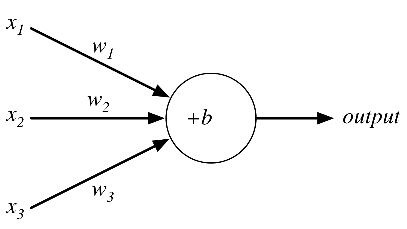
Consider the following perceptron:
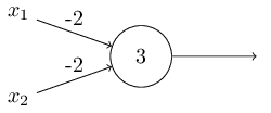
If $x$ takes on only binary values, what are the possible outputs?
Neurons

Instead of a binary output, we set the output to the result of an activation function $\sigma$
$$output = \sigma(w\cdot x + b)$$Activation Functions: Step (Perceptron)

Activation Functions: Sigmoid (Logistic)

Activation Functions: tanh

Activation Functions: ReLU
Rectified Linear Unit: $\sigma(z) = \max(0,z)$

Networks
Terminology alert: networks of neurons are sometimes called multilayer perceptrons, despite not using the step function.
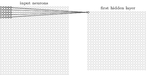
Networks
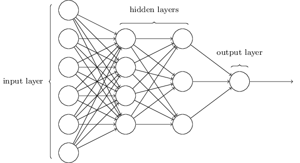
 The number of input neurons corresponds to the number of features.
The number of output neurons corresponds to the number of label classes. For binary classification, it is common to have two output nodes.
Layers are typically fully connected.
Neural Networks
The universal approximation theorem says that, if some reasonable assumptions are made, a feedforward neural network with a finite number of nodes can approximate any continuous function to within a given error $\epsilon$ over a bounded input domain.
The theorem says nothing about the design (number of nodes/layers) of such a network.
The theorem says nothing about the learnability of the weights of such a network.
These are open theoretical questions.
Given a network design, how are we going to learn weights for the neurons?
Stochastic Gradient Descent
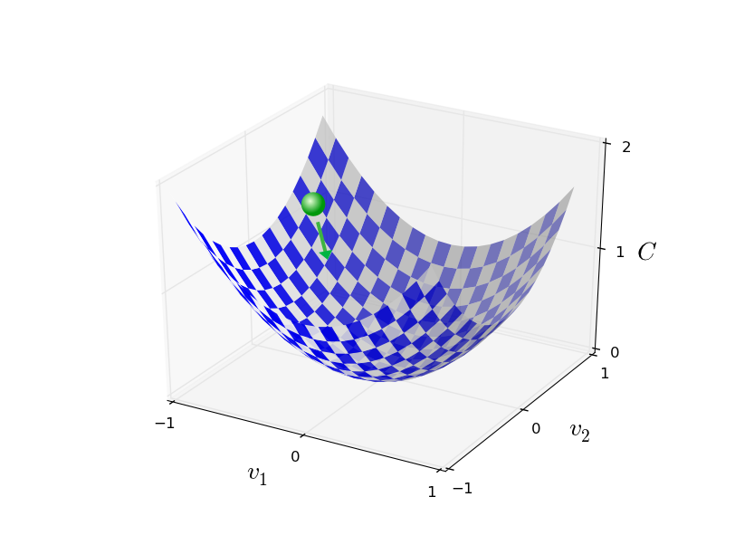
Randomly select $m$ training examples $X_j$ and compute the gradient of the loss function ($L$). Update weights and biases with a given learning rate $\eta$. $$ w_k' = w_k-\frac{\eta}{m}\sum_j^m \frac{\partial L_{X_j}}{\partial w_k}$$ $$b_l' = b_l-\frac{\eta}{m} \sum_j^m \frac{\partial L_{X_j}}{\partial b_l} $$
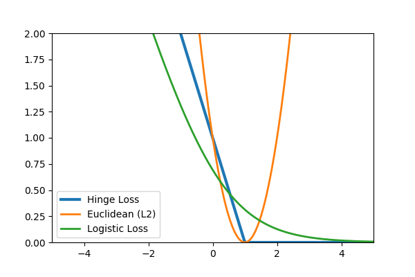
Common loss functions: logistic, hinge, cross entropy, euclidean
Backpropagation
Backpropagation is an efficient algorithm for computing the partial derivatives needed by the gradient descent update rule. For a training example $x$ and loss function $L$ in a network with $N$ layers:
Feedforward. For each layer $l$ compute $$a^{l} = \sigma(z^{l})$$ where $z$ is the weighted input and $a$ is the activation induced by $x$ (these are vectors representing all nodes of layer $l$).
Compute output error $$\delta^{N} = \nabla_a L \odot \sigma'(z^N)$$ where $ \nabla_a L_j = \partial L / \partial a^N_j$, the gradient of the loss with respect to the output activations. $\odot$ is the elementwise product.
Backpropagate the error $$\delta^{l} = ((w^{l+1})^T \delta^{l+1}) \odot \sigma'(z^{l})$$
Calculate gradients $$\frac{\partial L}{\partial w^l_{jk}} = a^{l-1}_k \delta^l_j \text{ and } \frac{\partial L}{\partial b^l_j} = \delta^l_j$$
Backpropagation as the Chain Rule
$$\frac{\partial L}{\partial a^l} \cdot \frac{\partial a^l}{\partial z^l} \cdot \frac{\partial z^l}{\partial a^{l-1}} \cdot \frac{\partial a^{l-1}}{\partial z^{l-1}} \cdot \frac{\partial z^{l-1}}{\partial a^{l-2}} \cdots \frac{\partial a^{1}}{\partial z^{l}} \cdot \frac{\partial z^{l}}{\partial x} $$
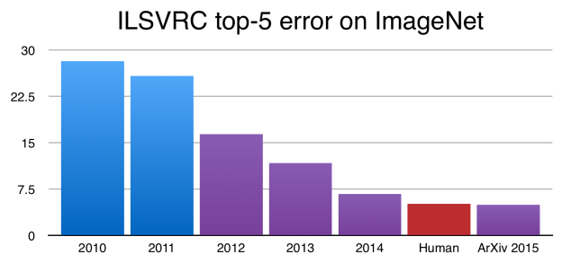
Deep Learning

A deep network is not more powerful (recall can approximate any function with a single layer), but may be more concise - can approximate some functions with many fewer nodes.
Convolution Filters
A filter applies a convolution kernel to an image.
The kernel is represented by an $n$x$n$ matrix where the target pixel is in the center.
The output of the filter is the sum of the products of the matrix elements with the corresponding pixels.
Examples from Wikipedia):
 |

|

|
| Identity | Blur | Edge Detection |
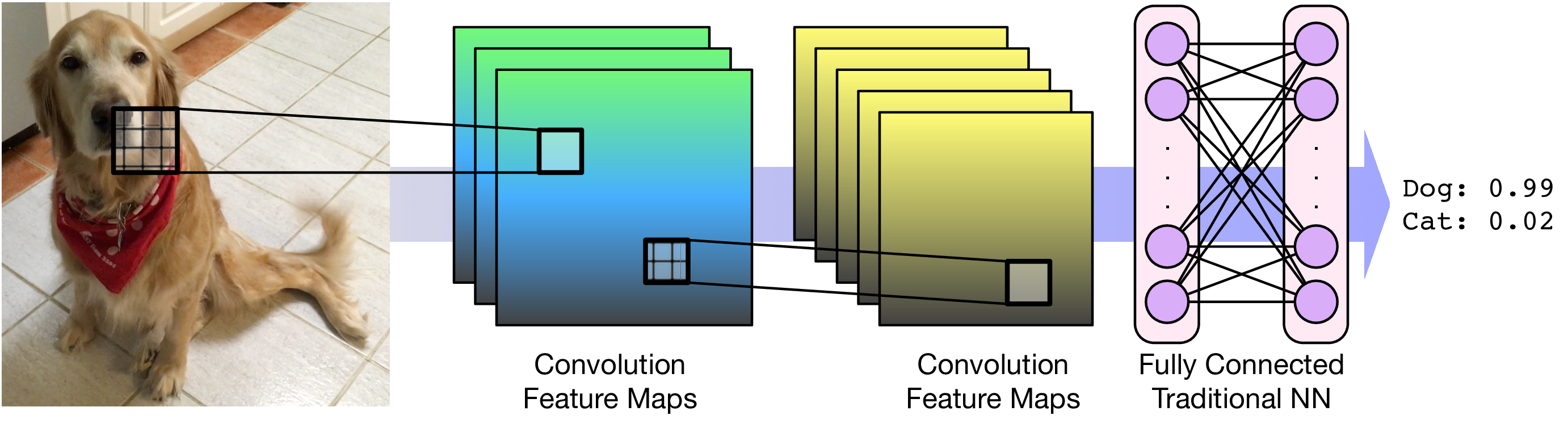
Feature Maps
We can think of a kernel as identifying a feature in an image and the resulting image as a feature map that has high values (white) where the feature is present and low values (black) elsewhere.
Feature maps retain the spatial relationship between features present in the original image.
Convolutional Layers
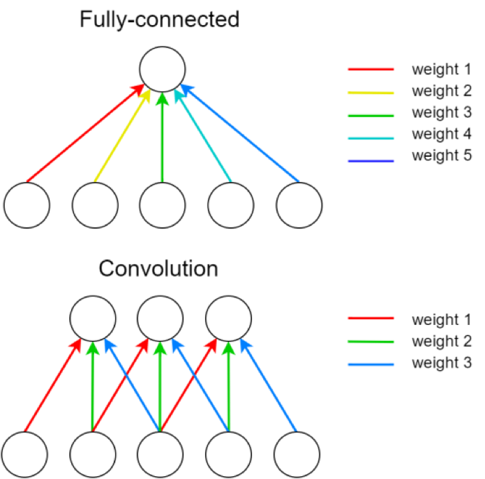 A single kernel is applied across the input. For each output feature map there is a single set of weights.
Convolutional Layers
For images, each pixel is an input feature. Each hidden layer is a set of feature maps.
Pooling
Pooling layers apply a fixed convolution (usually the non-linear MAX kernel). The kernel is usually applied with a stride to reduce the size of the layer.
- faster to train
- fewer parameters to fit
- less sensitive to small changes (MAX)

Consider an input image with 100 pixels. In a classic neural network, we hook these pixels up to a hidden layer with 10 nodes. In a CNN, we hook these pixels up to a convolutional layer with a 3x3 kernel and 10 output feature maps.
PyTorch Tensors
Tensor is very similar to numpy.array in functionality.
- Is allocated to a device (CPU vs GPU)
- Potentially maintains autograd information
Modules vs Functional
Modules are objects that can be initialized with default parameters and store any learnable parameters. Learnable parameters can be easily extracted from the module (and any member modules). Modules are called as functions on their inputs.
Functional APIs maintain no state. All parameters are passed when the function is called.
A network is a module
To define a network we create a module with submodules for operations with learnable parameters. Generally use functional API for operations without learnable parameters.
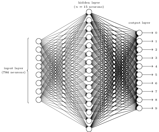
MNIST

Inputs need to be tensors...

Training MNIST
Training MNIST
Our network takes an image (as a tensor) and outputs class probabilities.
- Need a loss
- Need an optimizer (e.g. SGD, ADAM)
backwarddoes not update parameters
Training MNIST
Epoch - One pass through the training data.

This is the batch loss.
Testing MNIST
Some Failures
*Not from this particular network

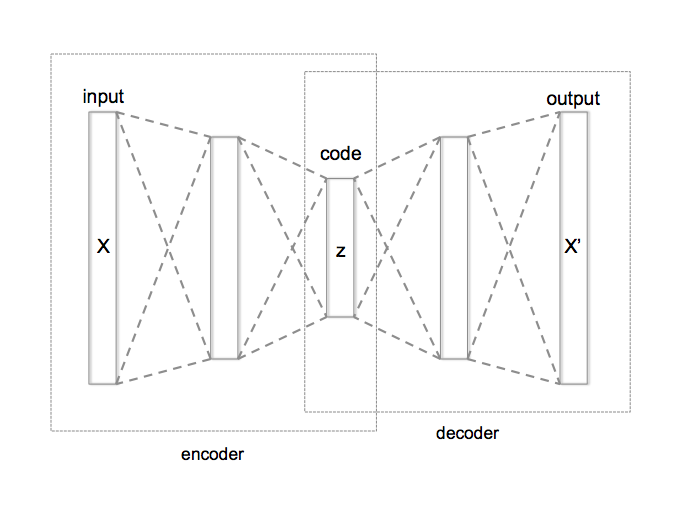
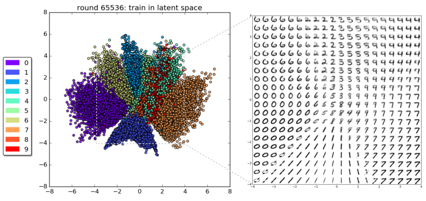
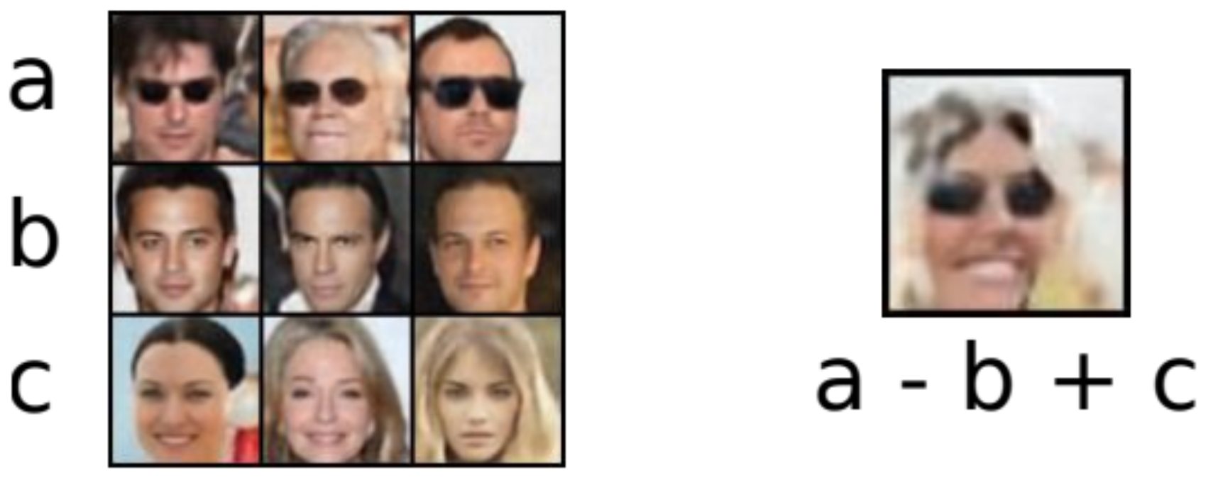
Generative vs. Discriminative
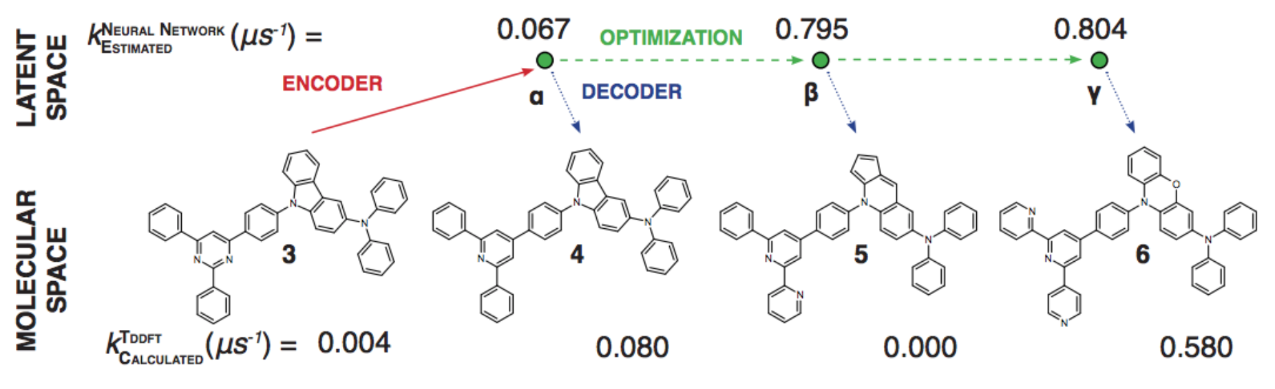
A generative model produces as output the input of a discriminative model: $P(X|Y=y)$ or $P(X,Y)$
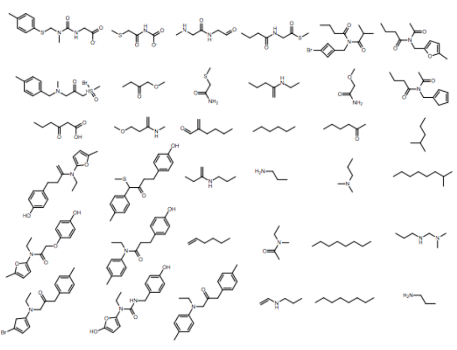
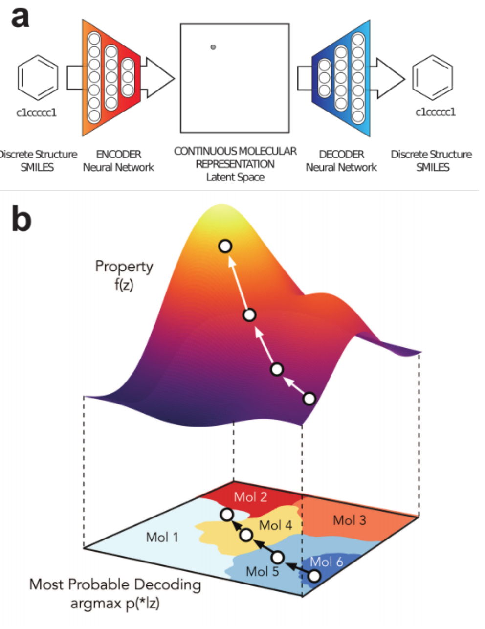 1% - 70% of output valid SMILES
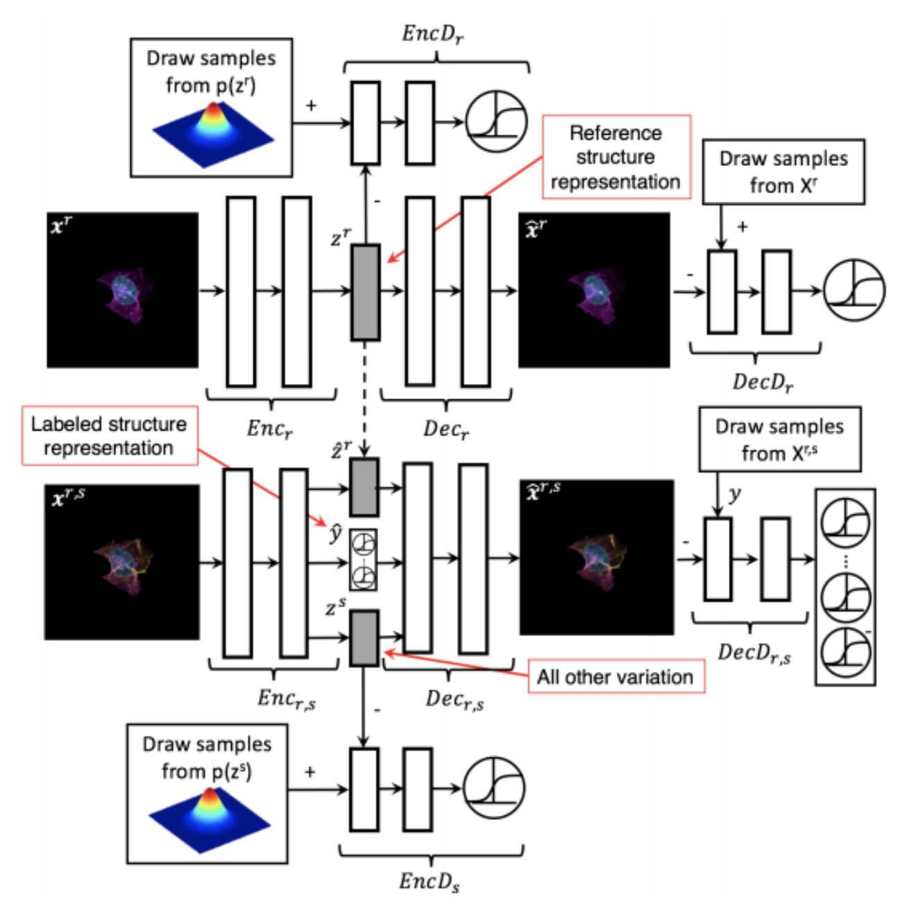
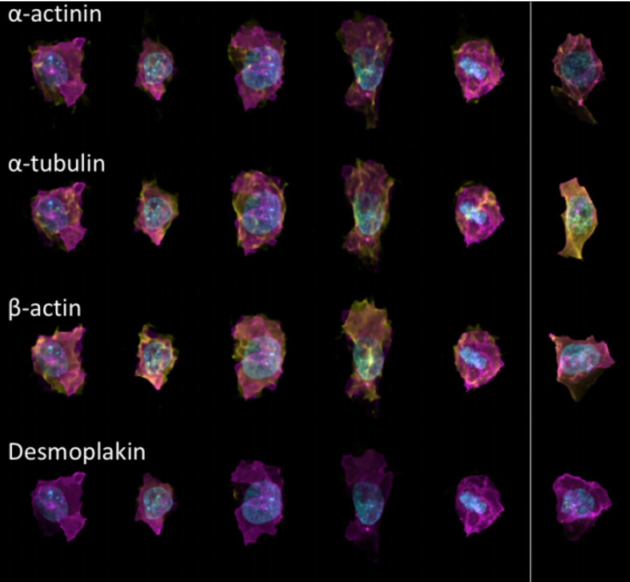
Generative Models of the Cell
https://arxiv.org/pdf/1705.00092.pdf
|
|
https://drive.google.com/file/d/0B2tsfjLgpFVhMnhwUVVuQnJxZTg/view
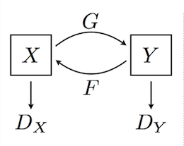
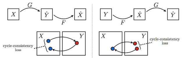
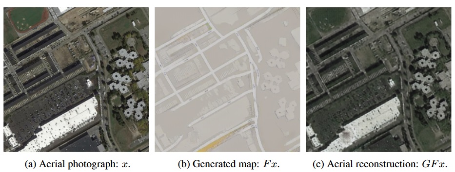
Generative Adversarial Networks
https://arxiv.org/abs/1406.2661
 https://youtu.be/G06dEcZ-QTg

Deep learning is not profound learning.
But it is quite powerful and flexible.